When Bigger Instances Don’t Scale

A bug hunt into why disk I/O performance failed to scale on larger AWS instances The promise of cloud computing is simple: more resources should equate to better, faster performance. When scaling up our systems by moving to larger instances, we naturally expect a proportional increase in capabilities, especially in critical areas like disk I/O. However, ScyllaDB’s experience enabling support for the AWS i7i and i7ie instance families uncovered a puzzling performance bottleneck. Contrary to expectations, bigger instances simply did not scale their I/O performance as advertised. This blog post traces the challenging, multi-faceted investigation into why IOTune (a disk benchmarking tool shipped with Seastar) was achieving a fraction of the advertised disk bandwidth on larger instances. On these machines, throughput plateaued at a modest 8.5GB/s and IOPS were much lower than expected on increasingly beefy machines. What followed was a deep dive into the internals of the ScyllaDB IO Scheduler, where we uncovered subtle bugs and incorrect assumptions that conspired to constrain performance scaling. Join us as we investigate the symptoms, pin down the root cause, and share the hard-fought lessons learned on this long journey. This blog post is the first in a three-part series detailing our journey to fully harness the performance of modern cloud instances. While this piece focuses on the initial set of bottlenecks within the IO Scheduler, the story continues in two subsequent posts. Part 2, The deceptively simple act of writing to disk, tracks down a mysterious write throughput degradation we observed in realistic ScyllaDB workloads after applying the fixes discussed here. Part 3, Common performance pitfalls of modern storage I/O, summarizes the invaluable lessons learned and provides a consolidated list of performance pitfalls to consider when striving for high-performance I/O on modern hardware and cloud platforms. Problem description Some time ago, ScyllaDB decided to support the AWS i7i and i7ie families. Before we support a new instance type, we run extensive tests to ensure ScyllaDB squeezes every drop of performance out of the provisioned hardware. While measuring disk capabilities with the Seastar IOTune tool, we noticed that the IOPS and bandwidth numbers didn’t scale well with the size of the instance, and we ended up with much lower values than AWS advertised. Read IOPS were on par with AWS specs up to i7i.4xlarge, but they were getting progressively worse, up to 25% lower than spec on i7i.48xlarge. Write IOPS were worse, starting at around 25% less than spec for i7i.4xlarge and up to 42% less on i7i.48xlarge. Bandwidth numbers were even more interesting. Our IOTune measurements were similar to fio up to the i7i.4xlarge instance type. However, as we scaled up the instance type, our IOTune bandwidth numbers were plateauing at around 8.5GB/s while fio was managing to pull up to 40GB/s throughput for i7i.48xlarge instances. Essential Toolkit The IOTune tool is a disk benchmarking tool that ships with Seastar. When you run this tool on a storage mount point, it outputs 4 values corresponding to the read/write IOPS and read/write bandwidth of the underlying storage system. These 4 values end up in a file called io-properties.yaml. When provided with these values, the Seastar IO Scheduler will build a model of the disk, which it will use to help ScyllaDB maximize the drive’s performance. The IO Scheduler models the disk based on the IOPS and bandwidth properties using a formula that looks something like: read_bw/read_bw_max + write_bw/write_bw_max + read_iops/read_iops_max + write_iops/write_iops_max <= 1 The internal mechanics of how the IO Scheduler works are described very thoroughly in the blog post I linked above. The io_tester tool is another utility within the Seastar framework. It’s used for testing and profiling I/O performance, often in more controlled and customizable scenarios than the automated IOTune. It allows users to simulate specific I/O workloads (e.g., sequential vs. random, various request sizes, and concurrency levels) and measure resulting metrics like throughput and latency. It is particularly useful for: Deep-dive analysis: Running experiments with fine-grained control over I/O parameters (e.g., --io-latency-goal, request size, parallelism) to isolate performance characteristics or potential bottlenecks. Regression testing: Verifying that changes to the IO Scheduler or underlying storage stack do not negatively impact I/O performance under various conditions. Fair Queue experimentation: As shown in this investigation, io_tester can be used to observe the relationship between configured workload parameters, the resulting in-disk queue lengths, and the throttling behavior of the IO Scheduler. What this meant for ScyllaDB We didn’t want to enable i7i instances if the IOTune numbers didn’t accurately reflect the underlying disk performance of the instance type. Lower io-properties numbers cause the IO Scheduler to overestimate the cost of each request. This leads to more throttling, making monstrous instances like i7i.48xlarge perform like much cheaper alternatives (such as the i7i.4xlarge, for example). Pinning the symptoms Early on, we noticed that the observed symptoms pointed to two different problems. This helped us narrow down the root causes much faster (well, fast here is a very misleading term). We were chasing a lower-than-expected IOPS issue and a different low-bandwidth issue. IOPS and bandwidth numbers were behaving differently when scaling up instances. The former was scaling, but with much lower values than we expected. The latter would just plateau from one point and stay there, no matter how much money you’d throw at the problem. We started with the hypothesis that IOTune might misdetect the disk’s physical block size from sysfs and that we issue requests with a different size than what the disk “likes,” leading to lower IOPS. After some debugging, we confirmed that IOTune indeed failed to detect the block size, so it defaulted to using requests of 512bytes. There’s no bug to fix on the IOTune side here, but we decided we needed to be able to specify the disk block size for reads and writes independently when measuring. This turned out to be quite helpful later on. With 4K requests, we were able to measure the expected ~1M IOPS for writes compared to the ~650k IOPS we were getting with the autodetected 512-byte requests (numbers relevant for the i7i.12xlarge instance). We had a fix for the IOPS issue, but – as we discovered later – we didn’t properly understand the actual root cause. At that point, we thought the problem was specific to this instance type and caused by IOTune misdetecting the block size. As you’ll see in the next blog post in the series, the root cause is a lot more interesting and complicated. The plateauing bandwidth issue was still on the table. Unfortunately, we had no clue about what could be going on. So, we started exploring the problem space, concentrating our efforts as you’d imagine any engineer would. Blaming the IO Scheduler We dug around, trying to see if IOTune became CPU-limited for the bandwidth measurements. But that wasn’t it. It’s somewhat amusing that our initial reaction was to point the finger at the IO Scheduler. This bias stems from when the IO Scheduler was first introduced in ScyllaDB. It had such a profound impact that numerous performance issues over time – things that were propagating downward to the storage team – were often (and sometimes unfairly) attributed to it. Understanding the root cause We went through a series of experiments to try to narrow down the problem further and hopefully get a better understanding of what was happening. Most of the experiments in this article, unless explicitly specified, were run on an i7i.12xlarge instance. The expected throughput was ~9.6GB/s while IOTune was measuring a write throughput of 8.5GB/s. 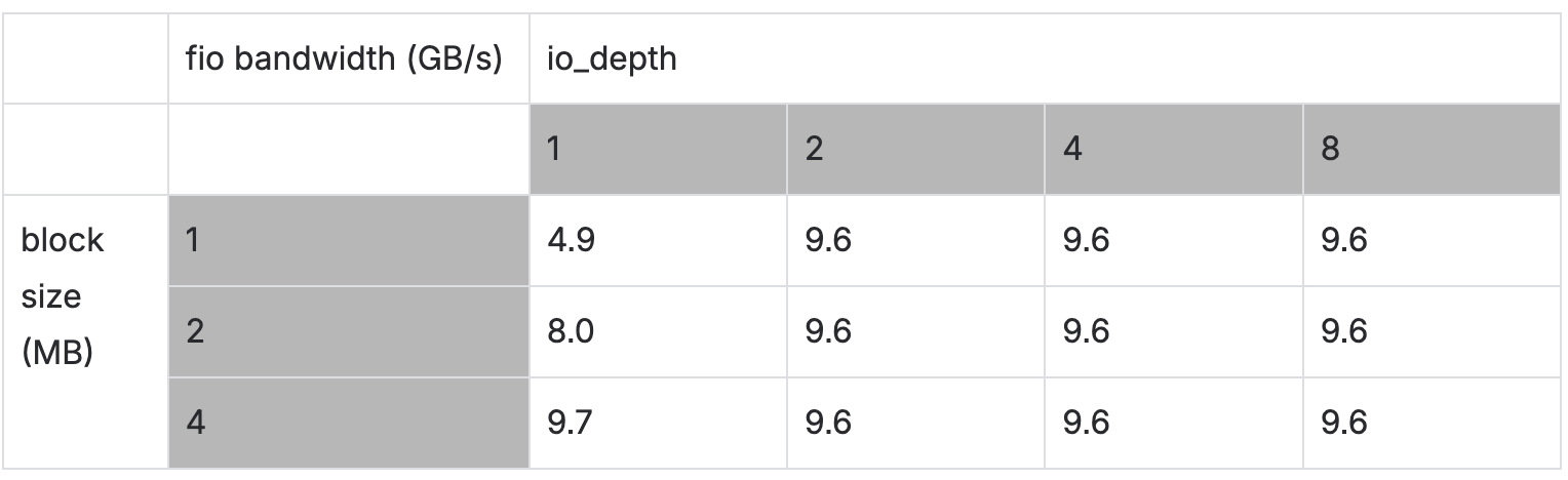To rule out poor disk queue utilization, we ran fio with various iodepths and block sizes, then recorded the bandwidth. We noticed that the request needs to be ~4MB to fill the disk queue. 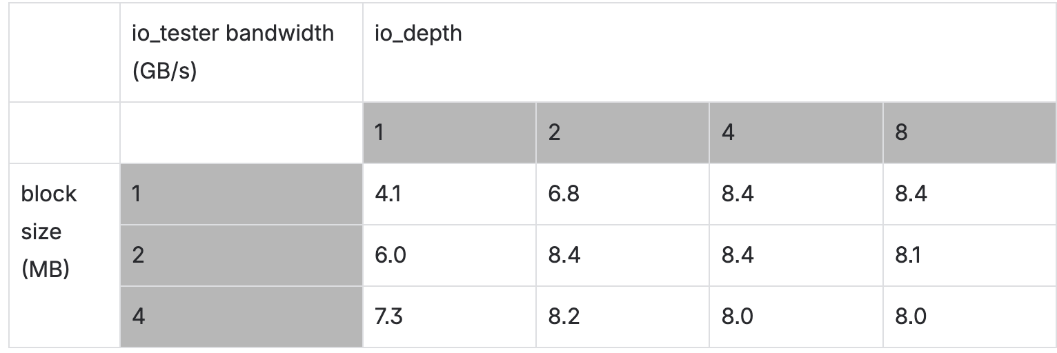Next, we collected the same for io_tester with –io-latency-goal=1000 to prevent the queue from splitting requests. A larger latency goal means the scheduler can be more relaxed and submit the requests as they come because it has plenty of time (1000 ms) to complete each request in time. If the goal is smaller, the IO Scheduler gets stressed because it needs to make each request complete in that tight schedule. Sometimes it might just split a request in half to take advantage of the in-disk parallelism and hopefully make the original request fit the tight latency goal. The fio tool seemed to be pulling the full bandwidth from the disk, but our io_tester tool was not. The issue was definitely on our side. The good news was that both io_tester and IOTune measured similar write throughputs, so we weren’t chasing a bug in our measurement tools. The conclusion of this experiment was that we saturated the disk queue properly, but we still got low bandwidth. Next, we pulled an ace out of the sleeve. A few months before this, we were at a hackathon during our engineering summit. During that hackathon, our Storage and Networking team built a prototype Seastar IO Scheduler controller that would bring more transparency and visibility into how the IO Scheduler works. One of the patches from that project was a hack that would make the IO Scheduler drop a lot of the IOPS/bandwidth throttling logic and just drain like crazy whatever requests are queued. We applied that patch to Seastar and ran the IOTune tool again. It was very rewarding to see the following output: Measuring sequential write bandwidth: 9775 MB/s (deviation 6%) Measuring sequential read bandwidth: 13617 MB/s (deviation 22%) The bandwidth numbers escaped the 8.5GB/s limit that was previously constraining our measurements. This meant we were correct in blaming the IO Scheduler. We were indeed experiencing throttling from the scheduler, specifically from something in the fair queue math. At that point, we needed to look more closely at the low-level behavior. We patched Seastar with another home-brewed project that adds a low-overhead binary tracer to the IO Scheduler. The plan was to run the tracer on both the master version and the one with the hackathon patch applied – then try to understand why the hackathon-patched scheduler performs better. 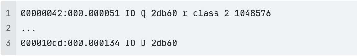We added a few traces and we immediately started to see patterns like these in the slow master trace: Here it took it 134-51=83us to dispatch one request. The “Q” event is when a request arrives at the scheduler and gets queued. “D” stands for when a request gets dispatched. For reference, the patched IO scheduler spent 1us to dispatch a request. The unexpected behavior suggested an issue with the token bucket accumulation, as requests should be dispatched instantly when running without io-properties.yaml (effectively providing unlimited tokens). This is precisely the scenario when IOTune is running: it withholds io-properties.yaml from the IO Scheduler. This allows the token bucket to operate with unlimited tokens, stressing the disk to its maximum potential so IOTune can compute, by itself, the required io-properties.yaml. The token bucket seems to run out of tokens…but why? When the token bucket runs out of tokens, it needs to wait for tokens to be replenished when other requests are completed. This delays the dispatch of the next request. That’s why the above request waited 83us to get dispatched when it should have actually been dispatched in 1us. There wasn’t much more we could do with the event tracer. We needed to get closer to the fair queue math. We returned to io_tester to examine the relationship between the parallelism of the test and the size of the in-disk queues. 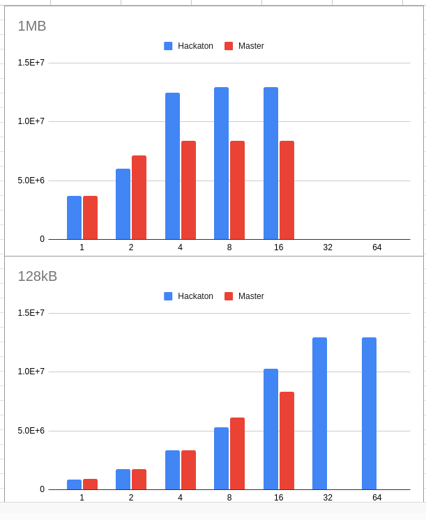We ran io_tester for requests sized within [128k, 1MB] with parallelism within [1,2,4,8,16] fibers. We ran it once for the master branch (slow) and once for the “hackathon” branch (fast). Here are some plots from these results. The plots are throughput (vertical axis) against parallelism (horizontal) for two request sizes, 1MB and 128kB. For both request sizes, the “hackathon” branch outperformed the “master” branch. Also, the 1MB request saturates the disk with much lower parallelism than the 128k request. No surprises here, the result wasn’t that valuable. 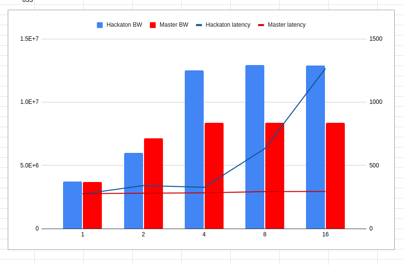In a follow-up test, we collected the in-disk latencies as well. We plotted throughput against parallelism for both the master and hackathon branches. The lines crossing the bars represent the in-disk latencies measured. This is already much better. After the disk is saturated, increasing parallelism should create a proportional increase for in-disk latency. That’s exactly what happens for the hackathon branch. We couldn’t say the same about the master branch. Here, the throughput plateaued around 4 fibers, and the in-disk latency didn’t grow! For some reason, we didn’t end up stressing this disk. 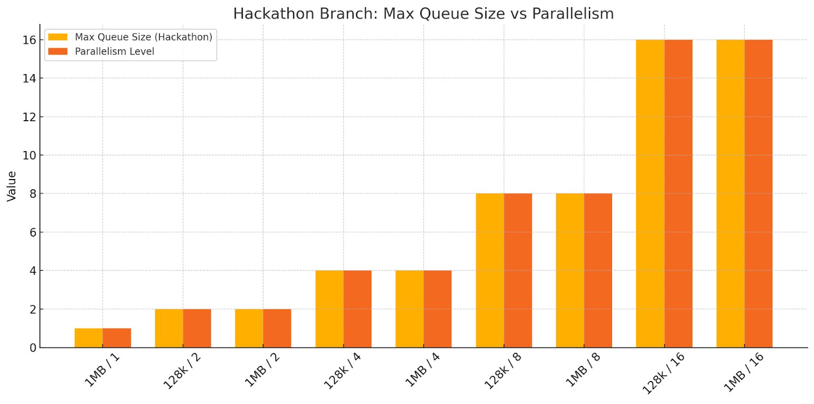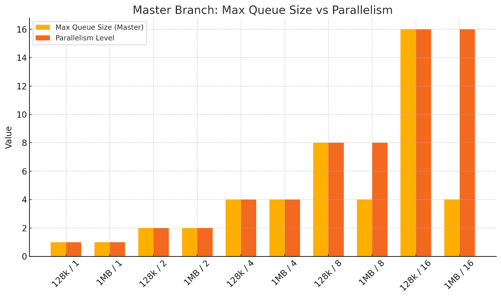To investigate further, we wanted to see the size of the actual in-disk queues. So, we coded up a patch to make io_tester output this information. We plotted the in-disk queue size alongside parallelism for various request sizes. At this point, it became clear that we weren’t sufficiently leveraging the in-disk parallelism. Likely, the fair_queue math was making the IO Scheduler throttle requests excessively. This is indeed what the plots below show. In the master (slow) branch run, the in-disk queue length for the 1MB request (which saturates the disk faster) plateaus at around 4 requests once parallelism=4 and higher. That’s definitely not alright. 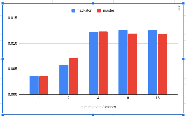Just for fun, let’s look at Little’s Law in action. We plotted disk_queue_length / latency for each branch as follows. Next, we wanted to (somehow) replicate this behavior without involving an actual disk. This way, we could maybe create a regression test for the IO Scheduler. 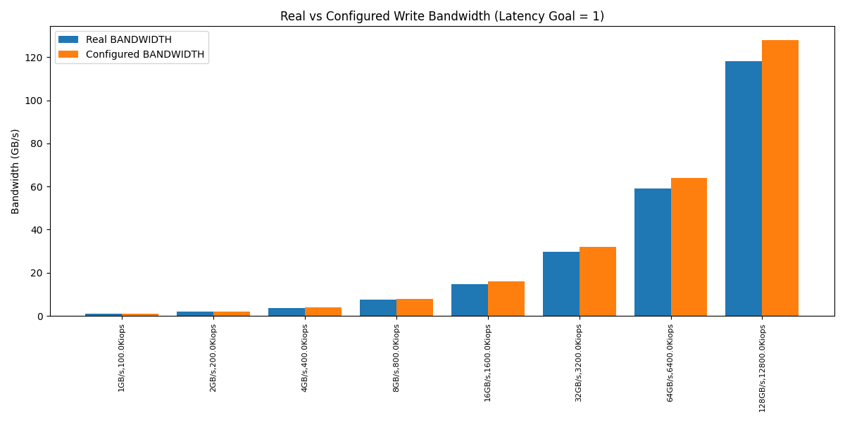The Seastar ioinfo tool was perfect for this job. ioinfo can take an io-properties.yaml file as an argument. It feeds the values to the IO Scheduler, then the tool outputs the token bucket parameters (which can be used to calculate the theoretical IOPS and throughput values that the IO Scheduler can achieve). Our goal was to compare these calculated values with what was configured in an io-properties.yaml file and make sure the IO Scheduler could deliver very close to what it was configured for. For reference, here’s how the calculated IOPS/bandwidth looked compared to the configured values. The values returned by the scheduler were within a 5% margin of the configured one. This was fantastic news (in a way). It meant the fair_queue math behaves correctly even with bandwidths above 8.xGB/s. We didn’t get the regression test we hoped for, since the fair_queue math was not causing the throttling and disk underutilization we’d seen in the previous experiment. However, we did add a test that would check if this behavior changes in the future. We did get a huge win from this, though. We came to the conclusion that something must be wrong with the fair_queue math or something in the IO Scheduler must be incorrect only when it’s not configured with an io-properties file. At that point, the problem space narrowed significantly. Playing around with the inputs from the io-properties.yaml file, we uncovered yet another bug. For large enough read IOPS/bandwidth numbers in the config file, the IO Scheduler would report request costs of zero. After many discussions, we learned that this is not really a bug. It’s how the math should behave. With big io-properties numbers, the math should plateau the costs at 0. It makes sense: the more resources you have available, the single unit of effort becomes less significant. This led us to an important realization: the unconfigured case (our original issue) should also produce a cost of zero. A zero cost means that the token bucket won’t consume any tokens. That gives us unbounded output…which is exactly what IOTune wants. Now we needed to figure out two things: Why doesn’t the IO Scheduler report a cost of zero for the unconfigured case? In theory, it should. In the issue linked above, costs became zero for values that weren’t even close to UINT64_MAX. Was our code prepared to handle costs of zero? We should ensure we don’t end up with weird overflows or divisions by zero or any undefined behavior from code that assumes costs can’t be zero. When things start to converge At this point, we had no further leads, so we thought there must be something wrong with the fair queue math. I reviewed the math from Implementing a New IO Scheduler Algorithm for Mixed Read/Write Workloads, but I didn’t find any obvious flaws that could explain our unconfigured case. We hoped we’d find some formula mistakes that made the bandwidth hit its theoretical limit at 8.5GB/s. We didn’t find any obvious issues here, so we concluded there must be some flaw in the implementation of the math itself. We started suspecting that there must be some overflow that ends up shrinking the bandwidth numbers. After quite some time tracking the math implementation in the code, we managed to find the issue. Two internal IO Scheduler variables that were storing the IOPS and bandwidth values configured via io-properties.yaml had a default value set to `std::numeric_limits<int>::max()`. It wasn’t that intuitive to figure out – the variables weren’t holding the actual io-properties values, but rather some values that derived from them. This made the mistake harder to spot. There is some code that recalculates those variables when the io-properties.yaml file is provided and parsed by the Seastar code. However, in the “unconfigured” case, those code paths are intentionally not hit. So, the INT_MAX values were carried into the fair queue math, crunched into the formulas, and resulted in the 8.xGB/s throughput limit we kept seeing. The fix was as simple as changing the default value to ‘std::numeric_limits<uint64_t>::max()’.  A one-line fix for many weeks of work. It’s been a crazy long journey chasing such a small bug, but it has been an invaluable (and fun!) learning experience. It led to lots of performance gains and enabled ScyllaDB to support highly efficient storage instances like i7i, i7ie and i8g. Stay tuned for the next episode in this series of blog posts, In part 2, we will uncover that the performance gains after this work weren’t quite what we were expecting on realistic workloads. We will deep dive into some very dark corners of modern NVMEs and filesystems to unlock a significant chunk of write throughput.