Scaling Performance Comparison: ScyllaDB Tablets vs Cassandra vNodes

Benchmarks show ScyllaDB tablet-based scaling 7.2× faster than Cassandra’s vNode-based scaling (9× with cleanup), sustaining ~3.5X higher throughput with fewer errors Real-world database deployments rarely experience steady traffic. Systems need sufficient headroom to absorb short bursts, perform maintenance safely, and survive unexpected spikes. At the same time, permanently sizing for peak load is wasteful. Elasticity lets you handle fluctuations without running an overprovisioned cluster. Increase capacity just-in-time when needed, then scale back as soon as the peak passes. When we built ScyllaDB just over a decade ago, it scaled fast enough for user needs at the time. However, deployments grew larger and nodes stored far more data per vCPU. Streaming took longer, especially on complex schemas that required heavy CPU work to serialize and deserialize data. The leaderless design forced operators to serialize topology changes, preventing parallel bootstraps or decommissions. And static (vNode-based) token assignments also meant data couldn’t be moved dynamically once a node was added. ScyllaDB’s recent move to tablet-based data distribution was designed to address those elasticity constraints. ScyllaDB now organizes data into independent tablets that dynamically split or merge as data grows or shrinks. Instead of being fixed to static ranges, tablets are load balanced transparently in the background to maintain optimal distribution. Clusters scale quickly with demand, so teams don’t need to overprovision ahead of time. If load increases, multiple nodes can be bootstrapped in parallel and start serving traffic almost immediately. Tablets rebalance in small increments, letting teams safely use up to ~90% of available storage. This means less wasted storage. The goal of this design is to make data movement more granular and reduce the serialized steps that constrained vNode-based scaling. To understand the impact of this design shift, we evaluated how both ScyllaDB (now using tablets) and Cassandra (still using vNodes) compare when they must increase capacity under active traffic. The goal was to observe scale-out under realistic conditions: workloads running, caches warm, and topology changes occurring mid-operation. By expanding both clusters step by step, we captured how quickly capacity came online, how much the running workload was affected, and how each system performed after each expansion. Before we go deeper into the details, here are the key findings from the tests: Bootstrap operations: ScyllaDB completed capacity expansion 7.2X faster than Cassandra Total scaling time: When including Cassandra’s required cleanup operations (which can be performed during maintenance windows), the time difference reaches 9X Throughput while scaling: ScyllaDB sustained ~3.5X more traffic during these scaling operations Stability under load: ScyllaDB had far fewer errors and timeouts during scaling, even at higher traffic levels Why Fast Scaling Matters Most real-world database deployments are overprovisioned to some extent. The extra capacity helps sustain traffic fluctuations and short-lived bursts. It also supports routine maintenance tasks, like applying security patches, rolling out infrastructure maintenance, or recovering from replica failures. Another important consideration in real-world deployments is that benchmark reports often overlook traffic variability over time. In practice, only a subset of workloads consistently demand high baseline throughput, with low variability from their peak needs. Most workloads follow a cyclical pattern, with daily peaks during active hours and significantly lower baseline traffic during off-hours. 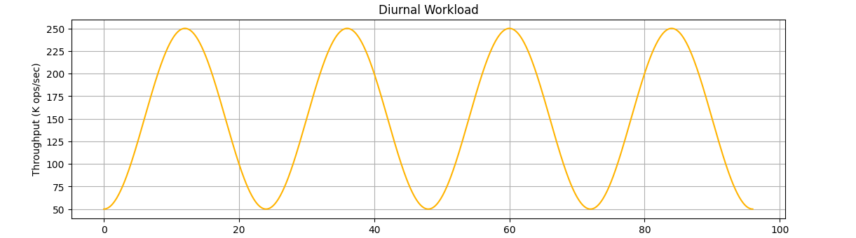A diurnal workload example, ranging between 50K to 250K operations per second in a day Fast scaling is also critical for handling unexpected events, such as viral traffic spikes, flash loads, backlog drains after cascading failures, or sudden pressure from upstream systems. It’s especially valuable when traffic has large peak-to-baseline swings, capacity needs to shift often, responses to load must be quick, or costs depend on scaling back down immediately after a surge. Comparing Tablets vs vNodes Fast scaling is ultimately a data distribution problem, and Cassandra’s vNodes and ScyllaDB’s tablets handle that distribution in distinctly different ways. Here’s more detail on the differences we previewed earlier. Apache Cassandra Apache Cassandra follows a token ring architecture. When a node joins the cluster, it is assigned a number of tokens (the default is 16), each representing a portion of the token ring. The node becomes responsible for the data whose partition keys fall within its assigned token ranges. During node bootstrap, existing replicas stream the relevant data to the new replica based on its token ownership. Conversely, when a node is removed, the process is reversed. Cassandra generally recommends avoiding concurrent topology changes; in practice, many operators add/remove nodes serially to reduce risk during range movements. Digression: In reality, topology changes in an Apache Cassandra cluster are plain unsafe. We explained the reasons in a previous blog, and pointed out that even its community acknowledged some of its design flaws. In addition to the administrative overhead involved in scaling a Cassandra cluster, there are other considerations. Adding nodes with higher CPU and memory is not straightforward. It typically requires a new tuning round and manually assigning a higher weight (increasing the number of tokens) to better match capacity. After bootstrap operations, Cassandra requires an intermediary step (cleanup) for older replicas in order to free up disk space and eliminate the risk of data resurrection. Lastly, multiple scaling rounds introduce significant streaming overhead since data is continuously shuffled across the cluster. 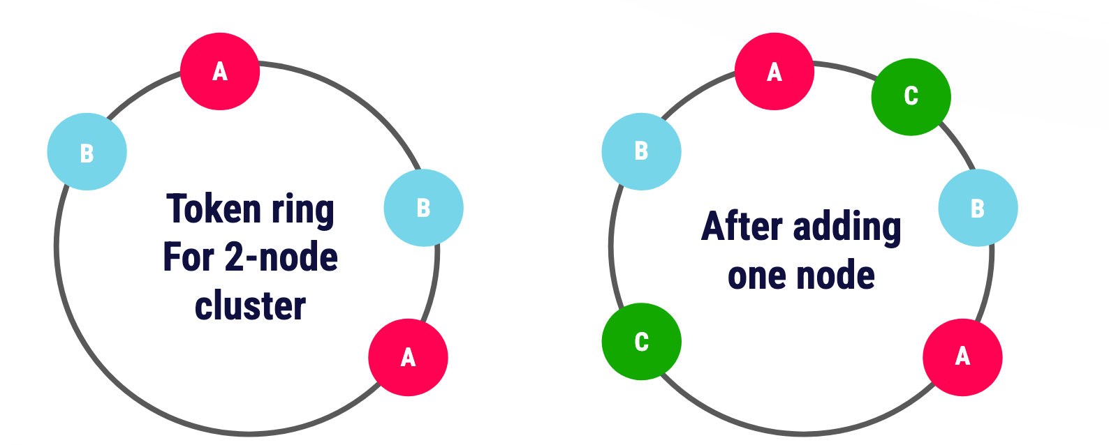Cassandra Token Ring ScyllaDB ScyllaDB introduced tablets starting with the 2024.2 release. Tablets are the smallest unit of replication in ScyllaDB and can be migrated independently across the cluster. Each table is dynamically split into tablets based on its size, with each tablet being assigned to a subset of replicas. In effect, tablets are smaller, manageable fragments of a table. As the topology evolves, tablet state transitions are triggered. A global load balancer balances tablets across the cluster, accounting for heterogeneity in node capacity (e.g., assigning more tablets to replicas with greater resources). Under the hood, Raft provides the underlying consensus mechanism that serializes tablet transitions in a way that avoids conflicting topology changes and ensures correctness. The load balancer is hosted on a single node, but not a designated node. If that node crashes or goes down for maintenance, the load balancer will start on another node. Raft and tablets effectively decouple topology changes from streaming operations. Users can orchestrate topology changes in parallel with minimal administrative overhead. ScyllaDB does not require a post-bootstrap cleanup phase. That allows for immediate request serving and more efficient data movement across the network. 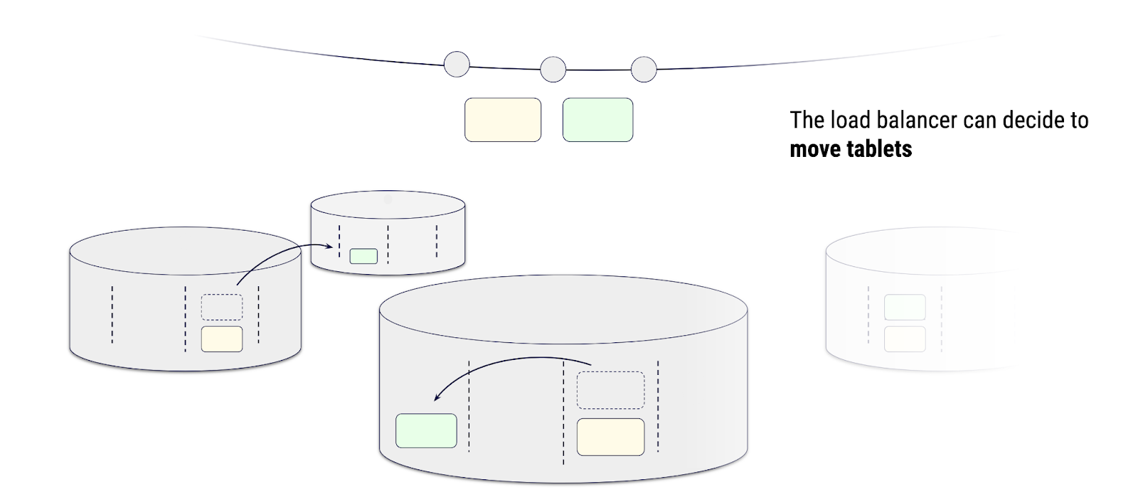Visual representation of tablets state transitions Adding Nodes Starting with a 3-node cluster, we ran our “real-life” mixed workload targeting 70% of each database’s inferred total capacity. Before any scaling activity, both ScyllaDB and Cassandra were warmed up to ensure disk and cache activity were in effect. Note: Configuration details are provided in the Appendix. We then started the mixed workload and let it run for another 30 minutes to establish a performance baseline. At this point, we bootstrapped 3 additional nodes, expanding the cluster to 6 nodes. We then allowed the workload to run for an additional 30 minutes to observe the effects of this first scaling step. We increased traffic proportionally. After sustaining it for another 30 minutes, we bootstrapped 3 more nodes, bringing each cluster to a total of 9 nodes. Finally, we increased traffic one last time to ensure each database could sustain its anticipated traffic. Note: See the Appendix for details on the test setup and our Cassandra tuning work. The following table shows the target throughput used during and after each scaling step along with each cluster’s inferred maximum capacity: Nodes ScyllaDB Cassandra 3 (baseline) 196K ops/sec (Max 280K) 56K ops/sec (Max 80K) 6 392K ops/sec (Max 560K) 112K ops/sec (Max 160K) 9 672K ops/sec (Max 840K) 168K ops/sec (Max 240K) We conducted this scaling exercise twice for each database, introducing a minor variation in each run. For ScyllaDB, we bootstrapped all 6 additional nodes in parallel. For Cassandra, we enabled both the Key Cache and Row Cache, as we observed it performed better overall under our initial performance results. 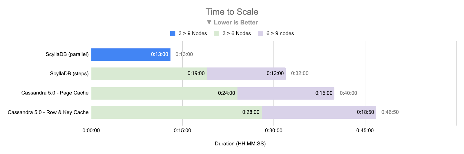Comparison of different scaling approaches At first glance, it might look like ScyllaDB offers only a modest improvement over Cassandra (somewhere between 1.25X and 3.6X faster). But there are deeper nuances to consider. Resiliency In both of our Cassandra benchmarks, we observed a high rate of errors, including frequent timeouts and OverloadedExceptions reported by the server. Notably, our client was configured with an exponential backoff, allowing up to 10 retries per operation. In this environment, both Cassandra configurations showed elevated error rates under sustained load during scaling. The following table summarizes the number of errors observed by the client during the tests: Kind Step Throughput Retries Cassandra 5.0 – Page Cache 3 → 6 nodes 56K ops/sec 2010 Cassandra 5.0 – Page Cache 6 → 9 nodes 112K ops/sec 0 Cassandra 5.0 – Row & Key Cache 3 → 6 nodes 56K ops/sec 5004 Cassandra 5.0 – Row & Key Cache 6 → 9 nodes 112K ops/sec 8779 With the sole exception of scaling from 6 to 9 nodes in the Page Cache scenario, all other Cassandra scaling exercises resulted in noticeable traffic disruption, even while handling 3.5X less traffic than ScyllaDB. In particular, the “Row & Key Cache” configuration proved itself unable to sustain prolonged traffic, ultimately forcing us to terminate that test prematurely. Performance The earlier comparison chart also highlights the cost of repeated streaming across incremental expansion steps. Although bootstrap duration is governed by the volume of data being streamed and decreases as more nodes are added, each scaling operation redundantly re-streams data that was already redistributed in prior steps. This introduces significant overhead, compounding both the time and performance of scaling operations. As demonstrated, scaling directly from 3 to 9 nodes using ScyllaDB tablets eliminates the intermediary incremental redistribution overhead. By avoiding redundant streaming at each intermediate step, the system performs a single, targeted redistribution of tablets, resulting in a significantly faster and more efficient bootstrap process. 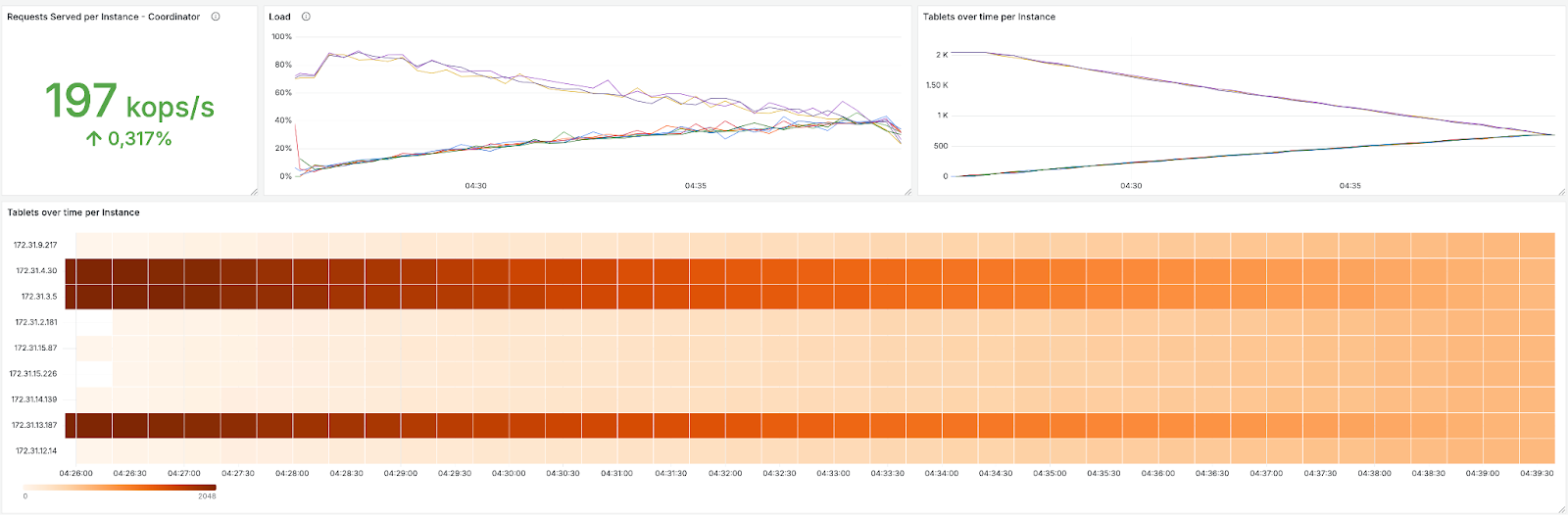ScyllaDB tablet streaming from 3 to 9 nodes After the scale out operations completed, we ran the following load tests to assess each database’s ability to withstand increased traffic: For ScyllaDB, we increased traffic to 80% of its peak capacity (280 * 3 * 0.8 = 672 Kops) For Cassandra, we increased traffic to 100% (240 Kops) and 125% (300 Kops) of its peak capacity to validate our starting assumptions 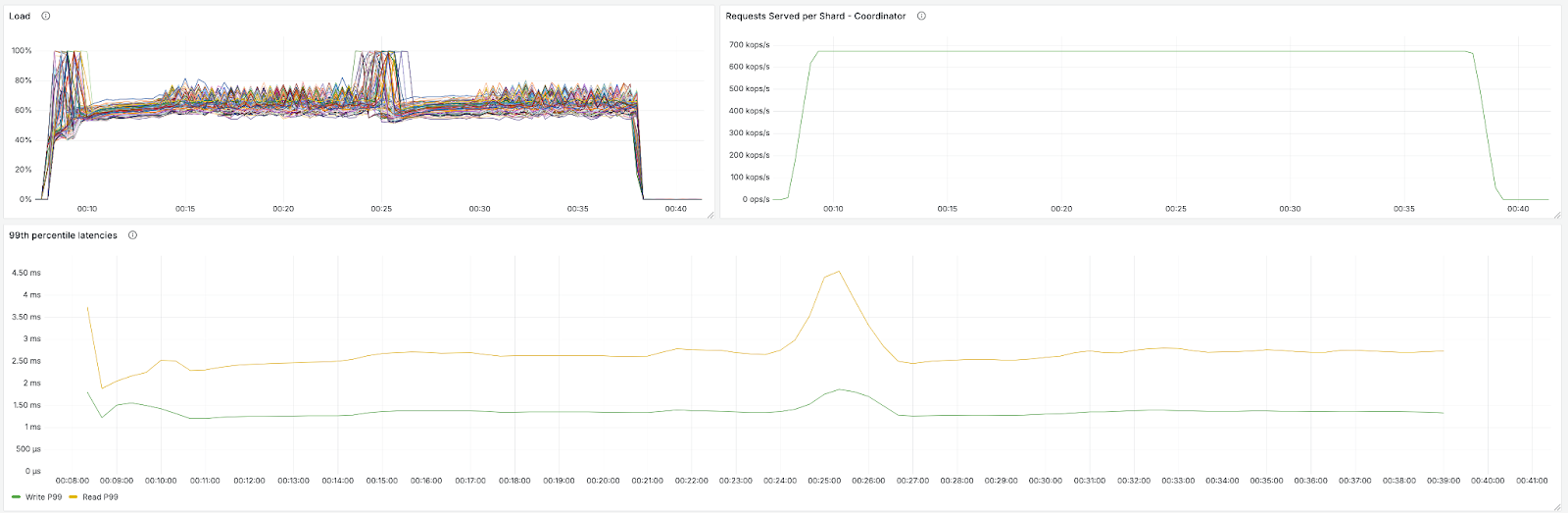ScyllaDB sustains 672 Kops/sec with load (per vCPU) around 80% utilization, as expected. 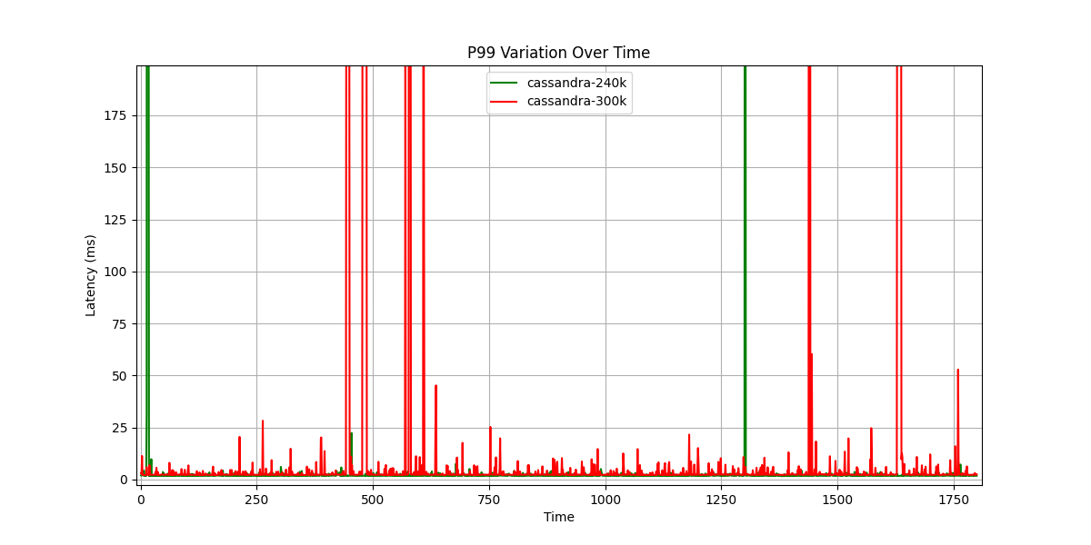Apache Cassandra latency variability under different throughput rates (240K vs 300K ops/sec) Cassandra maintained its expected 240K peak traffic. However, it failed to sustain 300K over time – leading to increased pauses and errors. This outcome was anticipated since the test was designed to validate our initial baseline assumptions, not to achieve or demonstrate superlinear scaling. Expectations In our tests, ScyllaDB scaled faster and delivered greater improvements in latency and throughput at each step. That reduces the number of scaling operations required. The compounded benefits translate to significantly faster capacity expansion. In contrast, Cassandra’s scaling behavior is more incremental. The initial scale-out from 3 to 6 nodes took 24 minutes. The subsequent step from 6 to 9 nodes introduced additional overhead, requiring 16 minutes. From this observation, we empirically derived a formula to model the scaling factor per step: 16 = 24 × (0.5/1.0)^overhead Solving for the exponent, we approximated the streaming overhead factor as 0.6. Using this, we constructed a practical formula to estimate Cassandra’s bootstrap duration at each scale step: Bootstrap_time ≈ Base_time × (data_to_stream / data_per_node)^0.6 With these formulas, we can project the bootstrap times for subsequent scaling steps. Based on our earlier performance results (where Cassandra sustained approximately 80K ops/sec for every 3-node increase), 27 total nodes of Cassandra would be required to match the throughput achieved by ScyllaDB. The following table presents the estimated cumulative bootstrap times needed for Cassandra to reach ScyllaDB performance, using the previously derived formula and applying the 0.6 streaming overhead factor at each step: Nodes Data to Stream Bootstrap Time Cumulative Time Peak Capacity 3 2.0TB – 0 min 80K 3 → 6 1.0TB 24.0 min 24.0 min 160K 6 → 9 0.67TB 15.8 min 39.8 min 240K 9 → 12 0.50TB 12.4 min 52.2 min 320K 12 → 15 0.40TB 10.4 min 62.6 min 400K 15 → 18 0.33TB 9.0 min 71.6 min 480K 18 → 21 0.29TB 8.1 min 79.7 min 560K 21 → 24 0.25TB 7.3 min 87.0 min 640K 24 → 27 0.22TB 6.7 min 93.7 min 720K   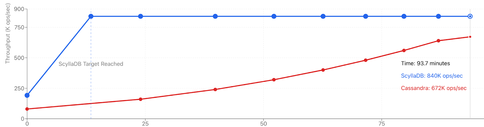Time to reach throughput capacity for bootstrap operations As the table and chart visually show, ScyllaDB responds to capacity needs 7.2X faster than Cassandra. That’s before accounting for the added operational and maintenance overhead associated with the process. Cleanup Cleanup is a process to reclaim disk space after a scale-out operation takes place in Cassandra. As the Cassandra documentation states: As a safety measure, Cassandra does not automatically remove data from nodes that “lose” part of their token range due to a range movement operation (bootstrap, move, replace). (…) If you do not do this, the old data will still be counted against the load on that node. 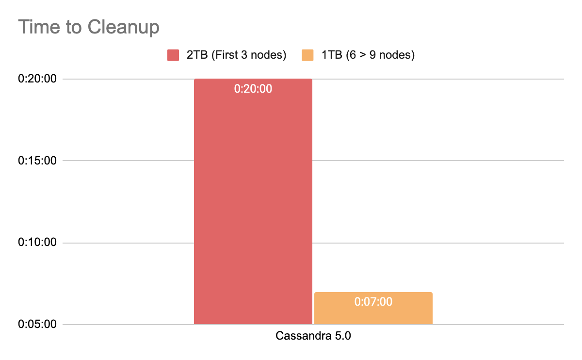We estimated the following cleanup times after scaling to 9 nodes with unthrottled compactions: Unlike topology changes, Cassandra cleanup operations can be executed in parallel across multiple replicas, rather than being serialized. The trade-off, however, is a temporary increase in compaction activity – something that may impact system performance through its execution. In practice, many users choose to run cleanup serially or per rack to minimize disruption to user-facing traffic. Despite its parallelizability, careful coordination is often preferred in production environments to minimize latency impact. 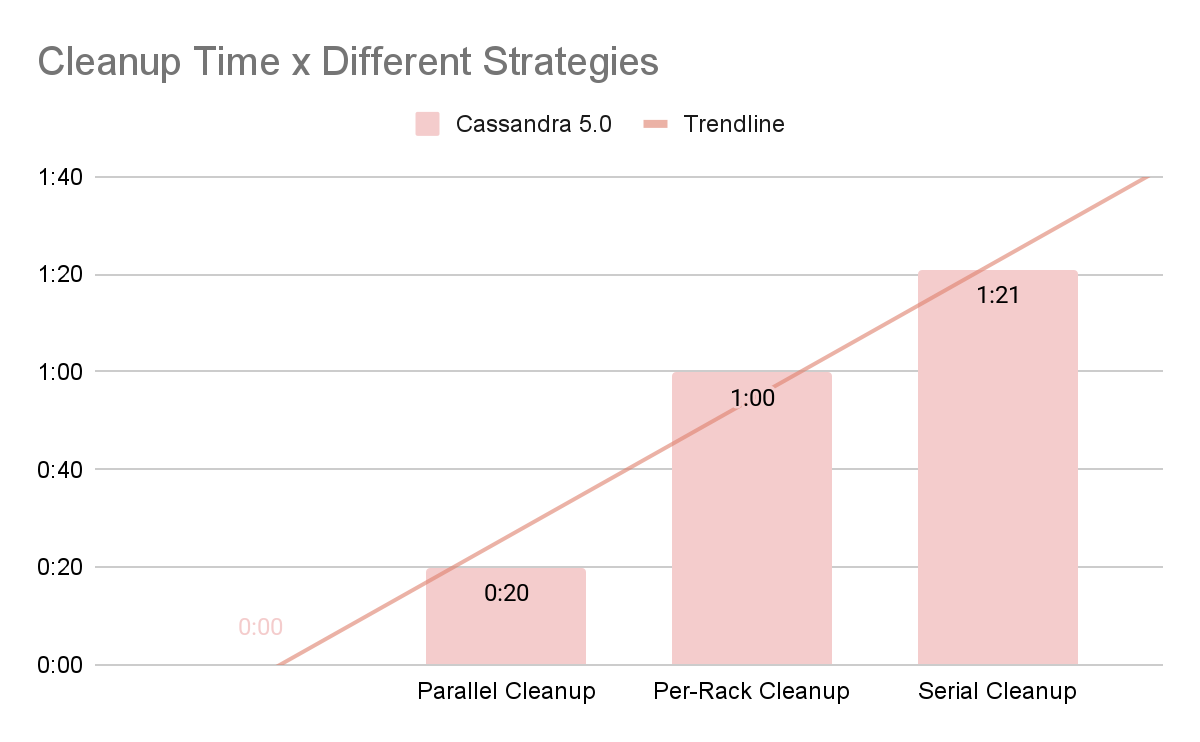The following table outlines the total time required under various cleanup strategies: In conclusion, ScyllaDB scaled faster and sustained higher throughput during scale-out, and it removes cleanup as part of the scaling cycle. Even for users willing to accept the risk of running cleanup in parallel across all Cassandra nodes, ScyllaDB still offers 9X faster capacity response time, once the minimum required cleanup time is factored into Cassandra’s previously estimated bootstrap durations. These results reflect how both databases behave under one specific scaling pattern. Teams should benchmark against their own workload shapes and operational constraints to see how these architectural differences play out in their particular environment. Parting Thoughts We know readers are (rightfully) skeptical of vendor benchmarks. As discussed earlier, Cassandra and ScyllaDB rely on fundamentally different scaling models, which makes designing a perfect comparison inherently difficult. The scaling exercises demonstrated here were not designed to fully maximize ScyllaDB tablets’ potential. The test design actually favors Cassandra by focusing on symmetrical scaling. Asymmetrical scaling scenarios would better highlight the advantage of tablets vs vNodes. Even with a design that favored Cassandra’s vNodes model, the results show the impact of tablets. ScyllaDB sustained 4X the throughput of Apache Cassandra while maintaining consistently lower P99 latencies under similar infrastructure. Interpreted differently, ScyllaDB delivers comparable performance to Cassandra using significantly smaller instances, which could then be scaled further by introducing larger, asymmetric nodes as needed. This approach (scaling from 3 small nodes to another 3 [much larger] nodes) optimizes infrastructure TCO and aligns naturally with ScyllaDB Tablets architecture. However, this would be far more difficult to achieve (and test) in Cassandra in practice. Also, the tests intentionally did not use large instances to avoid favoring ScyllaDB. ScyllaDB’s shard-per-core architecture is designed to linearly scale across large instances without requiring extensive tuning cycles, which are often encountered with Apache Cassandra. For example, a 3-node cluster running on the largest AWS Graviton4 instances can sustain over 4M operations per second. When combined with Tablets, ScyllaDB deployments can scale from tens of thousands to millions of operations per second within minutes. Finally, remember that performance should be just one component in a team’s database evaluation. ScyllaDB offers numerous features beyond Cassandra (local and global indexes, materialized views, workload prioritization, per query timeouts, internal cache, and advanced dictionary-based compression, for example). Appendix: How We Ran the Tests Both ScyllaDB and Cassandra tests were carried out in AWS EC2 in an apples-to-apples scenario. We ran our tests on a 3-node cluster running on top of i4i.4xlarge instances placed under the same Cluster Placement Group to further reduce networking round-trips. Consequently, each node was placed on an artificial rack using the GossipingPropertyFileSnitch. As usual, all tests used LOCAL_QUORUM as the consistency level, a replication factor of 3. They used NetworkTopologyStrategy as the replication strategy. To assess scalability under real-world traffic patterns, like Gaussian and other similar bell curve shapes, we measured the time required to bootstrap new replicas to a live cluster without disrupting active traffic. Based on these results, we derived a mathematical model to quantify and compare the scalability gaps between both systems. Methodology To assess scalability under realistic conditions, we ran performance tests to simulate typical production traffic fluctuations. The actual benchmarking is a series of invocations of ScyllaDB’s fork of latte with a consistency level of LOCAL_QUORUM. To test scalability, we used a “real-life” mixed distribution, with the majority (80%) of operations distributed over a hot set, and the remaining 20% iterating over a cold set. latte is the Lightweight Benchmarking Tool for Apache Cassandra as developed by Piotr Kołaczkowski, a DataStax Software Engineer. Under the hood, latte relies on ScyllaDB’s Rust driver, compatible with Apache Cassandra. It outperforms other widely used benchmarking tools, provides better scalability and has no GC pauses, resulting in less latency variability on the results. Unlike other benchmarking tools, latte (thanks to its use of Rune) also provides a flexible syntax for defining workloads closely tied on how developers actually interact with their databases. Lastly, we can always brag we did it in Rust, just because… 🙂 We set baseline traffic at 70% of its observed peak before P99 latency crossed a 10ms threshold. This was to ensure both databases retained sufficient CPU and I/O headroom to handle sudden traffic and concurrency spikes, as well as the overhead of scaling operations. Setup The following table shows the infrastructure we used for our tests: Cassandra/ScyllaDB Loaders EC2 Instance type i4i.4xlarge c6in.8xlarge Cluster size 3 1 vCPUs (total) 16 (48) 32 RAM (total) 128 (384) GiB 64 GiB Storage (total) 1 x 3.750 AWS Nitro SSD EBS-only Network Up to 25 Gbps 50 Gbps ScyllaDB and Cassandra nodes, as well as their respective loaders, were placed under their own exclusive AWS Cluster Placement Group for low-latency networking. Given the side-effect of all replicas being placed under the same availability zone, we placed each node under an artificial rack using the GossipingPropertyFileSnitch. The schema used through all testing suites resembles the same schema as the default cassandra-stress, whereas the keyspace relies on NetworkTopologyStrategy with a replication factor of 3:   CREATE TABLE IF NOT EXISTS keyspace1.standard1 (     key blob PRIMARY KEY,     c0 blob,     c1 blob,     c2 blob,     c3 blob,     c4 blob     ) ; We used a payload of 1010 bytes, where: 10-bytes represent the keysize, and; Each of the 5 columns is a distinct 200-byte blob Both databases were pre-populated with 2 billion partitions for an approximate (replicated) storage utilization of ~2.02TB. That’s about 60% disk utilization, considering the metadata overhead. Tuning Apache Cassandra Cassandra was originally designed to be run on commodity hardware. As such, one of its features is shipping with numerous different tuning options suitable for various use cases. However, this flexibility comes with a cost: tuning Cassandra is entirely up to its administrators, with limited guidance from online resources. Unlike ScyllaDB, an Apache Cassandra deployment requires users to manually tune kernel settings, set user limits, configure the JVM, set disks’ read-ahead, decide upon compaction strategies, and figure out the best approach for pushing metrics to external monitoring systems. To make things worse, some configuration file comments are outdated or ambiguous across versions. For example, CASSANDRA-16315 and CASSANDRA-7139 describe problems involving the default setting for concurrent compactors and offer advice on how to tune that parameter. Along those lines, it’s worth mentioning Amy Tobey’s Cassandra tuning guide (perhaps the most relevant Cassandra tuning resource available to date), where it says:   “The inaccuracy of some comments in Cassandra configs is an old tradition, dating back to 2010 or 2011. (…) What you need to know is that a lot of the advice in the config commentary is misleading. Whenever it says “number of cores” or “number of disks” is a good time to be suspicious. (…)” – Excerpt from Amy’s Cassandra tuning guide, cassandra.yaml section Tuning the JVM is a journey of its own. Cassandra 5.0 production recommendations don’t mention it, and the jvm-* files page only deals with the file-based structure as shipped with the database. Although DataStax’s Tuning Java resources does a better job on providing recommendations, it warns to adjust “settings gradually and test each incremental change.” Further, we didn’t find any references to ZGC (available as of JDK17) on either the Apache Cassandra or DataStax websites. That made us wonder whether this garbage collector was even recommended. Eventually, we settled on using settings similar to those that TheLastPickle used in their Apache Cassandra 4.0 Benchmarks. During our scaling tests, we hit another inconsistency: we noticed Cassandra’s streaming operations had a default cap of 24MiB/s per node, resulting in suboptimal transfer times. Upon raising those thresholds, we noticed that: Cassandra 4.0 docs mentioned tuning the stream_throughput_outbound_megabits_per_sec option Both Cassandra 4.1 and Cassandra 5.0 docs referenced the stream_throughput_outbound option This Instaclustr article (or carefully interpreting cassandra_latest.yaml) seem like the best resource for understanding the correct entire_sstable_stream_throughput_outbound option. In other words, 3 distinct settings exist for tuning the previous 3 major releases of Cassandra. If your organization is looking to upgrade, we strongly encourage you to conduct a careful review and full round of testing on your own. This is not an edge case; others noted similar upgrade problems under the Apache Cassandra Mailing List. CASSANDRA-20692 demonstrates that Apache Cassandra 5 failed to notice a potential WAL corruption under its newer Direct IO implementation, as issuing I/O requests without O_DSYNC could manifest as data loss during abrupt restarts. This, in turn, gives users a false sense of improved write performance. Configuring Apache Cassandra is not intuitive. We used cassandra_latest.yaml as a starting point, and ran multiple iterations of the same workload under a variety of settings and different GC settings. The results are shown below and demonstrate how little tuning can have a dramatic impact on Cassandra’s performance (for better or for worse). 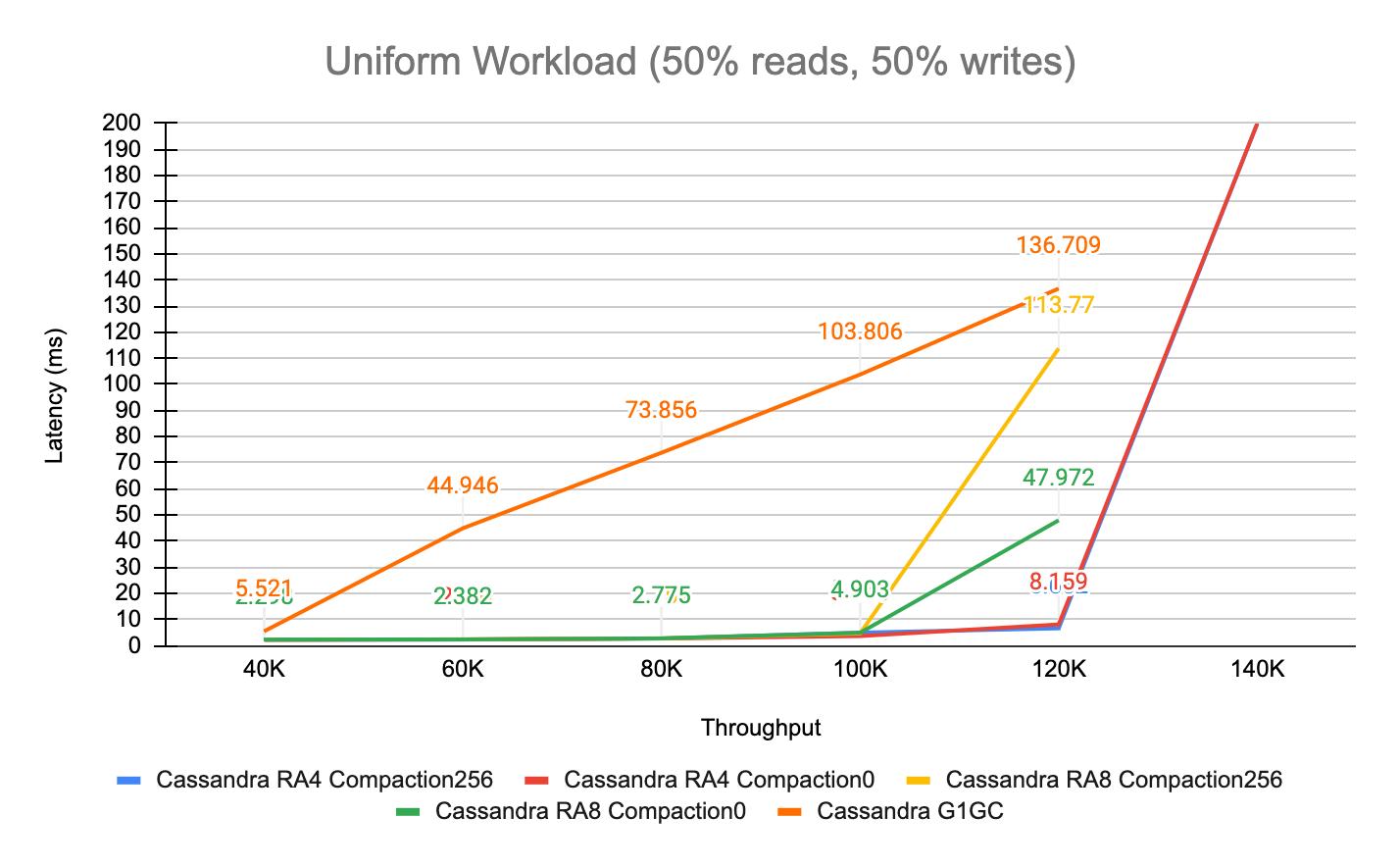We started by evaluating the performance of G1GC and observed that tail latencies were severely affected beyond a throughput of 40K/s. Simply switching to ZGC gave a nice performance boost, so we decided to stick with it for the remainder of our testing. The following table shows the performance variability of Cassandra 5.0 while using different tuning settings (it’s ordered from best to worst case): Test Kind Garbage Collector Read-ahead Compaction Throughput P99 Latency Throughput Cassandra RA4 Compaction256 ZGC 4KB 256MB/s 6.662ms 120K/s Cassandra RA4 Compaction0 ZGC 4KB Unthrottled 8.159ms 120K/s Cassandra RA8 Compaction256 ZGC 8KB 256MB/s 4.657ms 100K/s Cassandra RA8 Compaction0 ZGC 8KB Unthrottled 4.903ms 100K/s Cassandra G1GC G1GC 4KB 256MB/s 5.521ms 40K/s Although we spent a considerable amount of time tuning Cassandra to provide an unbiased and neutral comparison, we eventually found ourselves in a feedback loop. That is, the reported performance levels are only applicable for the workload being stressed running under the infrastructure in question. If we were to switch to different instance types or run different workload profiles, then additional tuning cycles would be necessary. We anticipate that the majority of Cassandra deployments do not undergo the level of testing we carried out on a per-workload basis. We hope that our experience may prevent other users from running into the same mistakes and gotchas that we did. We’re not claiming that our settings are the absolute best, but we don’t expect that further iterations will yield large performance improvements beyond what we observed. Tuning ScyllaDB We carried out very little tuning for ScyllaDB beyond what is described in the Configure ScyllaDB documentation. Unlike Apache Cassandra, the scylla_setup script takes care of most of the nitty-gritty details related to optimal OS tuning. ScyllaDB also used tablets for data distribution. We targeted a minimum of 100 tablets/shard with the following CREATE KEYSPACE statement: CREATE KEYSPACE IF NOT EXISTS keyspace1 WITH REPLICATION = { 'class': 'NetworkTopologyStrategy', 'datacenter1': 3 } AND tablets = {'enabled': true, 'initial': 2048}; Limitations of our Testing Performance testing often fails to capture real-world performance metrics tied to the semantics and access patterns of applications. Aspects such as variable concurrency, the impact of DELETEs (tombstones), hotspots, and large partitions were beyond the scope of our testing. Our work also did not aim to provide a feature-specific comparison. While Apache Cassandra 5.0 ships with newer (and less battle-tested) features like Storage-attached Indexes (SAI), ScyllaDB also ships with Workload Prioritization, Local Secondary Indexes, and Synchronous Materialized Views, all with no equivalent counterpart. However, we ensured both databases’ transparent and newer features were used, such as Cassandra’s Trie Memtables, Trie-indexed SSTables and its newer Unified Compaction Strategy, as well as ScyllaDB’s features like Tablets, Shard-awareness, SSTable Index Caching, and so forth. Future tests will use ScyllaDB’s Trie-indexed SSTables. Also note that both databases now offer Vector Search, which was not in scope for this project. Finally, this benchmark focuses specifically on scaling operations, not steady-state performance. ScyllaDB has historically demonstrated higher throughput and lower latency than Cassandra in multiple performance benchmarks. Cassandra 5 introduces architectural improvements, but our preliminary testing shows that ScyllaDB maintains its performance advantage. Producing a full apples-to-apples benchmark suite for Cassandra 5 is a sizable project that’s outside the scope of this study. For teams evaluating a migration, the best insights will come from testing your real-life workload profile, data models, and SLAs directly on ScyllaDB. If you are running your own evaluations (tip: ScyllaDB Cloud is the easiest way), our technical team can review your setup and share tips for accurately measuring ScyllaDB’s performance in your specific environment.