Contact Us
Contact Us
Read More
10 results found
Featured
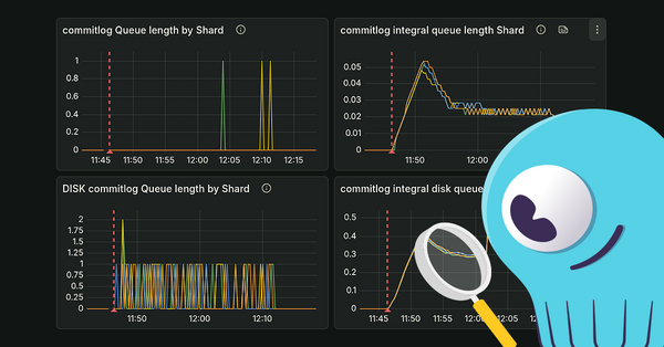
Integrated Gauges: Lessons Learned Monitoring Seastar's IO Stack - ScyllaDB
Featured
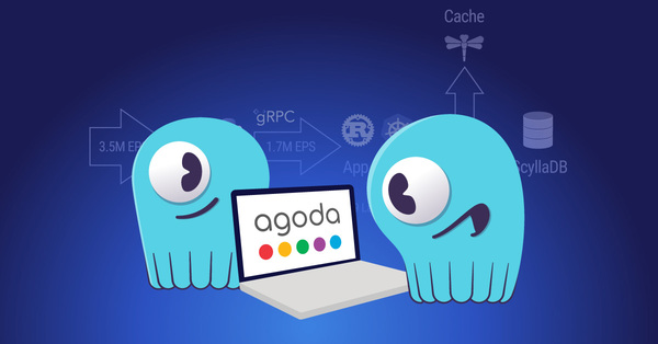
How Agoda Scaled Its Feature Store 50X
Featured
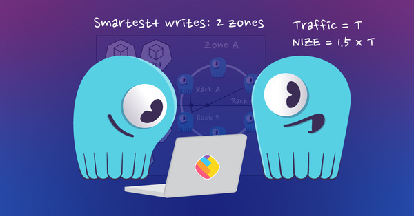
Optimizing a Fast Feature Store for Costs: Lessons Learned - ScyllaDB
Featured
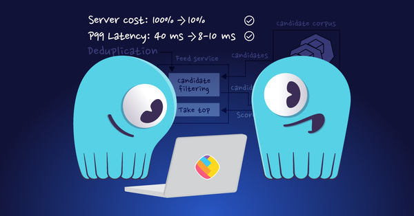
How ShareChat Cut Recommendation Engine Costs 90%, Step by Step
Featured
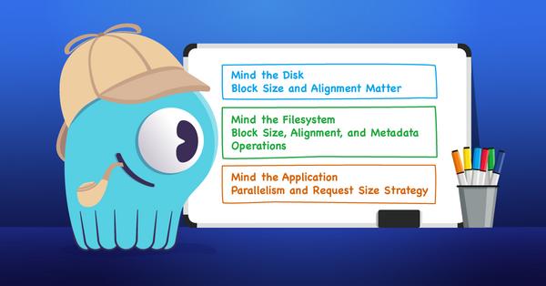
Common Performance Pitfalls of Modern Storage I/O
Featured
Kelsey Hightower’s Take on Engineering at Scale
Featured
The Deceptively Simple Act of Writing to Disk
Featured
We Built a Better Cassandra + ScyllaDB Driver for Node.js – with Rust
Featured
When Bigger Instances Don’t Scale
Featured
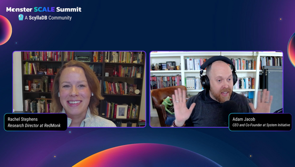
Scaling Is the “Funnest” Game: Rachel Stephens and Adam Jacob
Featured