Clues in Long Queues: High IO Queue Delays Explained

How seemingly peculiar metrics might provide interesting insights into system performance In large systems, you often encounter effects that seem weird at first glance, but – when studied carefully – give an invaluable clue to understanding system behavior. When supporting ScyllaDB deployments, we observe many workload patterns that reveal themselves in various amusing ways. Sometimes what seems to be a system misbehaving stems from a bad configuration or sometimes a bug in the code. However, pretty often what seems to be impossible at first sight turns into an interesting phenomenon. Previously we described one of such effects called “phantom jams.” In this post, we’re going to show another example of the same species. As we’ve learned from many of the ScyllaDB deployments we track, sometimes a system appears to be lightly loaded and only a single parameter stands out, indicating something that typically denotes a system bottleneck. The immediate response is typically to disregard the outlier and attribute it to spurious system slow-down. However, thorough and careful analysis of all the parameters, coupled with an understanding of the monitoring system architecture, shows that the system is indeed under-loaded but imbalanced – and that crazy parameter was how the problem actually surfaced. Scraping metrics Monitoring systems often follow a time-series approach. To avoid overwhelming their monitored targets and frequently populating a time-series database (TSDB) with redundant data, these solutions apply a concept known as a “scrape interval.” Although different monitoring solutions exist, we’ll mainly refer to Prometheus and Grafana throughout this article, given that these are what we use for ScyllaDB Monitoring. Prometheus polls its monitored endpoints periodically and retrieves a set of metrics. This is called “scraping”. Metrics samples collected in a single scrape consist of name:value pairs, where value is a number. Prometheus supports four core types of metrics, but we are going to focus on two of those: counters and gauges. Counters are monotonically increasing metrics that reflect some value accumulated over time. When observed through Grafana, the rate() function is applied to counters, as it reflects the changes since the previous scrape instead of its total accumulated value. Gauges, on the other hand, are a type of metric that can arbitrarily rise and fall. Apparently (and surprisingly at the same time) gauges reflect a metric state as observed during scrape-time. This effectively means that any changes made between scrape intervals will be overlooked, and are lost forever. Before going further with the metrics, let’s take a step back and look at what makes it possible for ScyllaDB to serve millions and billions of user requests per second at sub-millisecond latency. IO in ScyllaDB ScyllaDB uses the Seastar framework to run its CPU, IO, and Network activity. A task represents a ScyllaDB operation run in lightweight threads (reactors) managed by Seastar. IO is performed in terms of requests and goes through a two-phase process that happens inside the subsystem we call the IO scheduler. The IO Scheduler plays a critical role in ensuring that IO gets both prioritized and dispatched in a timely manner, which often means predictability – some workloads require that submitted requests complete no later than within a given, rather small, time. To achieve that, the IO Scheduler sits in the hot path – between the disks and the database operations – and is built with a good understanding of the underlying disk capabilities. To perform an IO, first a running task submits a request to the scheduler. At that time, no IO happens. The request is put into the Seastar queue for further processing. Periodically, the Seastar reactor switches from running tasks to performing service operations, such as handling IO. This periodic switch is called polling and it happens in two circumstances: When there are no more tasks to run (such as when all tasks are waiting for IO to complete), or When a timer known as a task-quota elapses, by default at every 0.5 millisecond intervals. The second phase of IO handling involves two actions. First, the kernel is asked for any completed IO requests that were made previously. Second, outstanding requests in the ScyllaDB IO queues are dispatched to disk using the Linux kernel AIO API. Dispatching requests into the kernel is performed at some rate that’s evaluated out of pre-configured disk throughput and the previously mentioned task-quota parameter. The goal of this throttled dispatching is to make sure that dispatched requests are completed within the duration of task-quota. Urgent requests that may pop up in the queue during that time don’t need to wait for the disk to be able to serve them. For the scope of this article, let’s just say that dispatching happens at the disk throughput. For example, if disk throughput is 10k operations per second and poll happens each millisecond, then the dispatch rate will be 10 requests per poll. IO Scheduler Metrics Since the IO Scheduler sits in the hot path of all IO operations, it is important to understand how the IO Scheduler is performing. In ScyllaDB, we accomplish that via metrics. Seastar exposes many metrics, and several IO-related ones are included among them. All IO metrics are exported per class with the help of metrics labeling, and each represents a given IO class activity at a given point in time. 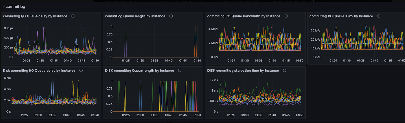IO Scheduler Metrics for the commitlog class Bandwidth and IOPS are two metrics that are easy to reason about. They show the rates at which requests get dispatched to disk. Bandwidth is a counter that gets increased by the request length every time it’s sent to disk. IOPS is a counter that gets incremented every time a request is sent to disk. When observed through Grafana, the aforementioned rate() function is applied and these counters are shown as BPS (bytes per second) and IO/s (IO per second), under their respective IO classes. Queue length metrics are gauges that represent the size of a queue. There are two kinds of queue length metrics. One represents the number of outstanding requests under the IO class. The other represents the number of requests dispatched to the kernel. These queues are also easy to reason about. Every time ScyllaDB makes a request, the class queue length is incremented. When the request gets dispatched to disk, the class queue length gauge is decremented and the disk queue length gauge is incremented. Eventually, as the IO completes, the disk queue length gauge goes down. When observing those metrics, it’s important to remember that they reflect the queue sizes as they were at the exact moment when they got scraped. It’s not at all connected to how large (or small) the queue was over the scrape period. This common misconception may cause one to end up with the wrong conclusions about how the IO scheduler or the disks are performing. Lastly, we have latency metrics known as IO delays. There are two of those – one for the software queue, and another for the disk. Each represents the average time requests spent waiting to get serviced. In earlier ScyllaDB versions, latency metrics were represented as gauges. The value shown was the latency of the last dispatched request (from the IO class queue to disk), or completed request (a disk IO completion). Because of that, the latencies shown weren’t accurate and didn’t reflect reality. A single ScyllaDB shard can perform thousands of requests per second and show the latency of a single request scraped after a long interval omits important insights about what really happened since the previous scrape. That’s why we eventually replaced these gauges with counters. Since then, latencies have been shown as a rate between the scrape intervals. Therefore, to calculate the average request delay, the new counter metrics are divided by the total number of IOPS dispatched within the scrape period. Disk can do more When observing IO for a given class, it is common to see corresponding events that took place during a specific interval. 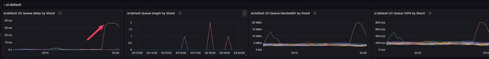Consider the following picture: IO Scheduler Metrics – sl:default class The exact numbers are not critical here. What matters is how different plots correspond to each other. What’s strange here? Observe the two rightmost panels – bandwidth and IOPS. On a given shard, bandwidth starts at 5MB/s and peaks at 20MB/s, whereas IOPS starts at 200 operations/sec and peaks at 800 ops. These are really conservative numbers. The system from which those metrics were collected can sustain 1GB/s bandwidth under several thousands IOPS. Therefore, given that the numbers above are per-shard, the disk is using about 10% of its total capacity. Next, observe that the queue length metric (the second from the left) is empty most of the time. This is expected, partially because it’s a gauge and it represents the number of requests sitting under the queue as observed during scrape time – but not the total number of requests which got queued. Since disk capacity is far from being saturated, the IO scheduler dispatches all requests to disk shortly after they arrive into the scheduler queue. Given that IO polling happens at sub-millisecond intervals, in-queue requests get dispatched to disk within a millisecond. So, why do the latencies shown in the queue delay metric (the leftmost one) grow close to 40 milliseconds? In such situations, ScyllaDB users commonly wonder, “The disk can do more – why isn’t ScyllaDB’s IO scheduler consuming the remaining disk capacity?!” IO Queue delays explained To get an idea of what’s going on, let’s simplify the dispatching model described above and then walk through several thought experiments on an imaginary system. Assume that a disk can do 100k IOPS, and ignore its bandwidth as part of this exercise. Next, assume that the metrics scraping interval is 1 second, and that ScyllaDB polls its queues once every millisecond. Under these assumptions, according to the dispatching model described above, ScyllaDB will dispatch at most 100 requests at every poll. Next, we’ll see what happens if servicing 10k requests within a second, corresponding to 10% of what our disk can handle. IOPS Capacity Polling interval Dispatch Rate Target Request Rate Scrape Interval 100K 1ms 100 per poll 10K/second 1s   Even request arrival In the first experiment, requests arrive evenly at the queue – one request at every 1/10k = 0.1 millisecond. By the end of each tick, there will be 10 requests in the queue, and the IO scheduler will dispatch them all to disk. When polling occurs, each request will have accumulated its own in-queue delays. The first request waited 0.9ms, the second 0.8ms, …, 0 ms. The sum results in approximately 5ms of total in-queue delay. After 1 second or 1K ticks/polls), we’ll observe a total in-queue delay of 5 seconds. When scraped, the metrics will be: A rate of 10K IOPS An empty queue An average in-queue delay/latency of 0.5ms (5 seconds total delay / 10K IOPS) Single batch of requests In the second experiment, all 10k requests arrive at the queue in the very beginning and queue up. As the dispatch rate corresponds to 100 requests per tick, the IO scheduler will need 100 polls to fully drain the queue. The requests dispatched at the first tick will contribute 1 millisecond each to the total in queue delay, with a total sum of 100 milliseconds. Requests dispatched at the second tick will contribute 2 milliseconds each, with a total sum of 200 milliseconds. Therefore, requests dispatched during the Nth tick will contribute N*100 milliseconds to the delay counter. After 100 ticks the total in-queue delay will be 100 + 200 + … + 10000 ms = 500000 ms = 500 seconds. Once the metrics endpoint gets scraped, we’ll observe: The same rate of 10k IOPS, the ordering of arrival won’t influence the result The same empty queue, given that all requests were dispatched in 100ms (prior to scrape time) 50 milliseconds in-queue delay (500 seconds total delay / 10K IOPS) Therefore, the same work done differently resulted in higher IO delays. Multiple batches If the submission of requests happens more evenly, such as 1k batches arriving at every 100ms, the situation would be better, though still not perfect. Each tick would dispatch 100 requests, fully draining the queue within 10 ticks. However, given our polling interval of 1ms, the following batch will arrive only after 90 ticks and the system will be idling. As we observed in the previous examples, each tick contributes N*100 milliseconds to the total in-queue delay. After the queue gets fully drained, the batch contribution is 100 + 200 + … + 1000 ms = 5000 ms = 5 seconds. After 10 batches, this results in 50 seconds of total delay. When scraped, we’ll observe: The same rate of 10k IOPS The same empty queue 5 milliseconds in-queue delay (50 seconds / 10K IOPS) To sum up: The above experiments aimed to demonstrate that the same workload may render a drastically different observable “queue delay” when averaged over a long enough period of time. It can be an “expected” delay of half-a-millisecond. Or, it can be very similar to the puzzle that was shown previously – the disk seemingly can do more, the software queue is empty, and the in-queue latency gets notably higher than the tick length. Average queue length over time Queue length is naturally a gauge-type metric. It frequently increases and decreases as IO requests arrive and get dispatched. Without collecting an array of all the values, it’s impossible to get an idea of how it changed over a given period of time. Therefore, sampling the queue length between long intervals is only reliable in cases of very uniform incoming workloads. There are many parameters of the same nature in the computer world. The most famous example is the load average in Linux. It denotes the length of the CPU run-queue (including tasks waiting for IO) over the past 1, 5 and 15 minutes. It’s not a full history of run-queue changes, but it gives an idea of how it looked over time. Implementing a similar “queue length average” would improve the observability of IO queue length changes. Although possible, that would require sampling the queue length more regularly and exposing more gauges. But as we’ve demonstrated above, accumulated in-queue total time is yet another option – one that requires a single counter, but still shows some history. Why is a scheduler needed? Sometimes you may observe that doing no scheduling at all may result in much better in-queue latency. Our second experiment clearly shows why. Consider that – as in that experiment, 10k requests arrive in one large batch and ScyllaDB just forwards them straight to disk in the nearest tick. This will result in a 10000 ms total latency counter, respectively 1ms average queue delay. The initial results look great. At this point, the system will not be overloaded. As we know, no new requests will arrive and the disk will have enough time and resources to queue and service all dispatched requests. In fact, the disk will probably perform IO even better than it would while being fed eventually with requests. Doing so would likely maximize the disk’s internal parallelism in a better way, and give it more opportunities to apply internal optimizations, such as request merging or batching FTL updates. So why don’t we simply flush the whole queue into disk whatever length it is? The answer lies in the details, particularly in the “as we know” piece. First of all, Seastar assigns different IO classes for different kinds of workloads. To reflect the fact that different workloads have different importance to the system, IO classes have different priorities called “shares.” It is then the IO scheduler’s responsibility to dispatch queued IO requests to the underlying disk according to class shares value. For example, any IO activity that’s triggered by user queries runs under its own class named “statement” in ScyllaDB Open Source, and “sl:default” in Enterprise. This class usually has the largest shares denoting its high priority. Similarly, any IO performed during compactions occurs in the “compaction” class, whereas memtable flushes happen inside the “memtable” class – and both typically have low shares. We say “typically” because ScyllaDB dynamically adjusts shares of those two classes when it detects more work is needed for a respective workflow (for example, when it detects that compaction is falling behind). Next, after sending 10k requests to disk, we may expect that they will all complete in about 10k/100k = 100ms. Therefore, there isn’t much of a difference whether requests get queued by the IO scheduler or by the disk. The problem happens if and only if a new high-priority request pops up when we are waiting for the batch to get serviced. Even if we dispatch this new urgent request instantly, it will likely need to wait for the first batch to complete. Chances that disk will reorder it and service earlier are too low to rely upon, and that’s the delay the scheduler tries to avoid. Urgent requests need to be prioritized accordingly, and get served much faster. With the IO Scheduler dispatching model, we guarantee that a newly arrived urgent request will get serviced almost immediately. Conclusion Understanding metrics is crucial for understanding the behavior of complex systems. Queues are an essential element present in any data processing, and seeing how data traverses through queues is crucial for engineers solving real-life performance problems. Since it’s impossible to track every single data unit, compound metrics like counters and gauges become great companions for achieving said task. Queue length is a very important parameter. Observing its change over time reveals bottlenecks of the system, thus shedding light on performance issues that can arise in complex highly loaded systems. Unfortunately, one cannot see the full history of queue length changes (like you can with many other parameters), and this results in a misunderstanding of the system behavior. This article described an attempt to map queue length from gauge-type metrics to a counter-type one – thus making it possible to accumulate a history of the queue length changes over time. Even though the described “total delay” metrics and its behavior is heavily tied to how ScyllaDB monitoring and Seastar IO scheduler work, this way of accumulating and monitoring latencies is generic enough to be applied to other systems as well. More ScyllaDB Engineering Blogs