Contact Us
Contact Us
Read More
10 results found
Featured
ScyllaDB Vector Search Benchmark: 10M Vectors on a Compact Cluster - ScyllaDB
Featured
Shrinking the Search: Introducing ScyllaDB Vector Quantization - ScyllaDB
Featured
Why We Changed ScyllaDB’s Approach to Repair - ScyllaDB
Featured
ScyllaDB R&D Year in Review: Elasticity, Efficiency, and Real-Time Vector Search - ScyllaDB
Featured
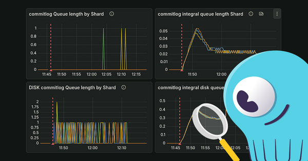
Integrated Gauges: Lessons Learned Monitoring Seastar's IO Stack - ScyllaDB
Featured
Demo: ScyllaDB Engineering in Action
Featured
The Future of Data Consistency in ScyllaDB
Featured
The Path to Tiered Storage
Featured
ScyllaDB Flow Control: As Fast as Possible, But Not Faster
Featured
Efficient Data Consistency: Incremental Repair for ScyllaDB Tablets
Featured