Compression in ScyllaDB

This article was published in 2019
This blog focuses on the problem of storing as much information as we can in the least amount of space as possible. The first part will deal with the basics of compression theory and implementations in ScyllaDB. The second part will look at actual compression ratios and performance.
Part 1: The basics of compression theory and implementations in ScyllaDB
First, let’s look at a basic example of compression. Here’s some information for you:
Piotr Jastrzębski is a developer at ScyllaDB. Piotr Sarna is a developer at ScyllaDB. Kamil Braun is a developer at ScyllaDB.
And here’s the same information, but taking less space:
Piotr Jastrzębski#0. Piotr Sarna#0. Kamil Braun#0.0: is a developer atScyllaDB.
I compressed the data using a lossless algorithm. If you knew the algorithm I used, you’d be able to retrieve the original string from the latter string, i.e. decompress it. For our purposes we will only consider lossless algorithms.
We would like to apply compression to the files we store on our disk to make them smaller with the possibility of retrieving the original files later.
First, let's focus on the theory behind compression: what makes compression possible, and what sometimes doesn’t; what are the general ideas used in the algorithms supported by ScyllaDB; and how is compression used to make SSTables smaller.
Next, we’ll look at a couple of benchmarks that compare the different supported algorithms to help us understand which ones are better suited for which situations: why should we use one for cases where latency is important, and why should we use the other for cases where lowering space usage is crucial.
Lossless compression
Unfortunately, one does not simply compress any file and expect that the file will take less space after compression. Consider the set of all strings of length 5 over the alphabet {0, 1}:
A = {00000, 00001, 00010, 00011, …, 11110, 11111}.
Suppose that we have 32 (25) files on our disk, each taking 5 bits, each storing a different sequence from the above set. We would like to take our latest, bleeding-edge technology, better-than-everyone-else compression algorithm, and apply it to our files so that each file takes 4 or fewer bits after compression. And, of course, we want the compression to be lossless. In other words, we want to have an injective function from our set A to the set of strings of length <= 4 over {0, 1}:
B = {0, 1, 00, 01, 10, 11, 100, …, 1110, 1111}
The function is the compression algorithm. Injectivity means that no two elements from A will be mapped to the same element in B, and that’s what makes the compression lossless. But that’s just not possible, because the cardinality of A is 32, while the cardinality of B is 31. A German mathematician named Dirichlet once said (paraphrasing): if you try to put n pigeons into n - 1 holes, then at least one hole will be shared by two pigeons. That rule is known as the pigeonhole principle.  The pigeonhole principle as illustrated on Wikipedia. Therefore any lossless algorithm that makes some inputs smaller after compression, makes other inputs at least as big after compression as the input itself. So which inputs shall be made smaller?
Complexity
Try to understand the difference between the following two strings. First:
0000000011111111,
Second:
001100000100101.
To create the first string, I invented a simple rule: eight 0s first, then eight 1s. For the second string, I threw a coin 16 times (really).
A person asked on the street would say that the second string is “more random” than the first. An experienced mathematician would say that the second string has greater Kolmogorov complexity (probably).
Kolmogorov complexity, named after the Russian mathematician Kolmogorov, is a fun concept. The (Kolmogorov) complexity of a string is the length of the shortest program which outputs the string and terminates. By “outputs the string” we mean a program that takes no input and outputs the string each time it is executed (so we don’t count random programs which sometimes output a different string). To be completely precise we would have to specify what exactly a “program” means (usually we use Turing machines for that). Intuitively, strings of lower complexity are those that can be described using fewer words or symbols.
Returning to our example, try to describe our two strings in English in as few words as possible. Here’s my idea for the first one: “eight zeros, eight ones”. And for the second one, I’d probably say “two zeros, two ones, five zeros, one, two zeros, one, zero, one”. Send me a message if you find something much better. :-)
Intuitively, strings of high complexity should be harder to compress. Indeed, compression tries to achieve exactly what we talked about: creating shorter descriptions of data. Of course I could easily take a long, completely random string and create a compressor which outputs a short file for this particular string by hard-coding the string inside the compressor. But then, as explained in the previous section, other strings would have to suffer (i.e. result in bigger files), and the compressor itself would become more complex by remembering this long string. If we’re looking to develop compressors that behave well on “real-world” data, we should aim to exploit structure in the encountered strings — because the structure is what brings complexity down.
But the idea of remembering data inside the compressor is not completely wrong. Suppose we knew in advance we’ll always be dealing with files that store data related to a particular domain of knowledge — we expect these files to contain words from a small set. Then we don’t care if files outside of our interest get compressed badly. We will see later that this idea is used in real-world compressors.
Unfortunately, computing Kolmogorov complexity is an undecidable problem (you can find a short and easy proof on Wikipedia). That’s why the mathematician from above would say “probably.”
To finish the section on complexity, here’s a puzzle: in how many words can we describe the integer that cannot be described in fewer than twelve words?
Compressing SSTables
ScyllaDB uses compression to store SSTable data files. The latest release supports 3 algorithms: LZ4, Snappy, and DEFLATE. Recently another algorithm, Zstandard, was added to the development branch. We’ll briefly describe each one and compare them in later sections.
What compression algorithm is used, if any, is specified when creating a table. By default, if no compression options are specified for a table, SSTables corresponding to the table will be compressed using LZ4. The following commands are therefore equivalent:
create table t (a int primary key, b int) with compression = {'sstable_compression': 'LZ4Compressor'};create table t (a int primary key, b int);.
You can check the compression options used by the table using a describe table statement. To disable compression you’d do:
create table t (a int primary key, b int) with compression =
{'sstable_compression': ''};
A quick reminder: in ScyllaDB, rows are split into partitions using the partition key. Inside SSTables, partitions are stored continuously: between two rows belonging to one partition there cannot be a row belonging to a different partition.
This enables performing queries efficiently. Suppose we have an uncompressed table t with integer partition key a, and we’ve just started ScyllaDB, so there’s no data loaded into memtables. When we perform a query like the following:
select * from t where a = 0;then in general we don’t need to read each of the SSTables corresponding to t entirely to answer that query. We only need to read each SSTable from the point where partition a = 0 starts to the point where the partition ends. Obviously, to do that, we need to know the positions of partitions inside the file. ScyllaDB uses partition summaries and partition indexes for that.
Things get a bit more complicated when compression is involved (but not too much). If we had compressed the entire SSTable, we would have to decompress it entirely to read the desired data. This is because the concept of order of data does not exist inside the compressed file. In general, no piece of data in the original file corresponds to a particular piece in the compressed file — the resulting file can only be understood by the decompression algorithm as one whole entity.
Therefore ScyllaDB splits SSTables into chunks and compresses each chunk separately. The size of each chunk (before compression) is specified during table creation using the chunk_length_in_kb parameter:
create table t (a int primary key, b int) with compression =
{‘sstable_compression’: ‘LZ4Compressor’, ‘chunk_length_in_kb’: 64};
By the way, the default chunk length is 4 kilobytes.
Now to read a partition, an additional data structure is used: the compression offset map. Given a position in uncompressed data it tells the partition index which chunk corresponds to (contains) the position.
There is a tradeoff that the user should be aware of. When dealing with small partitions, large chunks may significantly slow down reads, since to read even a small partition, the entire chunk containing it (or chunks, if the partition happens to start at the end of one chunk) must be decompressed. On the other hand, small chunks may decrease the space efficiency of the algorithm (i.e., the compressed data will take more space in total). This is because a lot of compression algorithms (like LZ4) perform better the more data they see (we explain further below why that is the case).
Algorithms supported by ScyllaDB
LZ4 and Snappy focus on compression and decompression speed, therefore they are well suited for low latency workloads. At the same time they provide quite good compression ratios. Both algorithms were released in 2011. LZ4 was developed by Yann Collet, while Snappy was developed at, and released by Google.
Both belong to the LZ77 family of algorithms, meaning they use the same core approach for compression as the LZ77 algorithm (described in a paper published in 1977). The differences mostly lie in the format of the compressed file and in the data structures used during compression. Here I’ll only briefly describe the basic idea used in LZ77.
The string
abcdefgabcdeabcde
would be described by a LZ77-type algorithm as follows:
abcdefg(5,7)(5,5)
How the shortened description is then encoded in the compressed file depends on the specific algorithm.
The decompressor reads the description from left to right, remembering the decompressed string up to this point. Two things can happen: either it encounters a literal, like abcdefg, in which case it simply appends the literal to the decompressed string, or it encounters a length-distance pair (l,d), in which case it copies l characters at offset d behind the current position, appending them to the decompressed string.
In our example, here are the steps the algorithm would make:
- Start with an empty string,
- Append abcdefg (current decompressed string: abcdefg),
- Append 5 characters at 7 letters behind the current end of the decompressed string, i.e., append abcde (current string: abcdefgabcde),
- Append 5 characters at 5 letters behind the current end of the decompressed string, i.e., append abcde (current string: abcdefgabcdeabcde).
We see that the compressor must find suitable candidates for the length-distance pairs. Therefore a LZ77-type algorithm would read the input string from left to right, remembering some amount of the most recent data (called the sliding window), and use it to replace encountered duplicates with length-distance pairs. Again, the exact data structures used are a detail of the specific algorithm.
Now we can also understand why LZ4 and Snappy perform better on bigger files (up to a limit): the chance to find a duplicated sequence of characters to be replaced with a length-distance pair increases the more data we have seen during compression.
DEFLATE and ZStandard also build on the ideas of LZ77. However, they add an extra step called entropy encoding. To understand entropy encoding, we first need to understand what prefix codes (also called prefix-free codes) are.
Suppose we have an alphabet of symbols, e.g. A = {0, 1}. A set of sequences of symbols from this alphabet is called prefix-free if no sequence is a prefix of the other. So, for example, {0, 10, 110, 111} is prefix-free, while {0, 01, 100} is not, because 0 is a prefix of 01.
Now suppose we have another alphabet of symbols, like B = {a, b, c, d}. A prefix code of B in A is an injective mapping from B to a prefix-free set of sequences over A. For example:
a -> 0, b -> 10, c -> 110, d -> 111
is a prefix code from B to A.
The idea of entropy encoding is to take an input string over one alphabet, like B, and create a prefix code into another alphabet, like A, such that frequent symbols are assigned short codes while rare symbols are assigned long codes.
Say we have a string like “aaaaaaaabbbccd”. Then the encoding written earlier would be a possible optimal encoding for this string (another optimal encoding would be a -> 0, b -> 10, c -> 111, d -> 110).
It’s easy to see how entropy coding might be applied to the problem of file compression: take a file, split it into a sequence of symbols (for example, treating every 8-bit sequence as a single symbol), compute a prefix code having the property mentioned above, and replace all symbols with their codes. The resulting sequence, together with information on how to translate the codes back to the original alphabet, will be the compressed file.
Both DEFLATE and ZStandard begin with running their LZ77-type algorithms, then apply entropy encoding to the resulting shortened descriptions of the input files. The alphabet used for input symbols and the entropy encoding method itself is specific to each of the algorithms. DEFLATE uses Huffman coding, while ZStandard combines Huffman coding with Finite State Entropy.
DEFLATE was developed by Phil Katz and patented in 1991 (the patent expired in 2019). However, a later specification in RFC 1951 said that “the format can be implemented readily in a manner not covered by patents.“ Today it is a widely adopted algorithm implemented, among other places, in the zlib library and used in the gzip compression program. It achieves high compression ratios but can be a lot slower during compression than LZ4 or Snappy (decompression remains fast though) — we will see an example of this in benchmarks included in part two of this blog. Therefore, in ScyllaDB, DEFLATE is a good option for workloads where latency is not so important but we want our SSTables to be as small on disk as possible.
In 2016 Yann Collet, author of LZ4, released the first version of zstd, the reference C implementation of the ZStandard algorithm. It can achieve compression ratios close to those of DEFLATE, while being competitive on the speed side (although not as good as LZ4 or Snappy).
Remember how we talked about storing data inside the compressor to make it perform better with files coming from a specific domain? ZStandard enables its users to do that with the option of providing a compression dictionary, which is then used to enhance the duplicate-removing part of the algorithm. As you’ve probably guessed, this is mostly useful for small files. Of course the same dictionary needs to be provided for both compression and decompression.
Part 1 Conclusions
We have seen why not everything can be compressed due to the pigeonhole principle and looked at Kolmogorov complexity, which can be thought of as a mathematical formalization of the intuitive concept of “compressibility”. We’ve also described how compression is applied to SSTables in a way that retains the possibility of reading only the required parts during database queries. Finally, we’ve discussed the main principles behind the LZ77 algorithm and the idea of entropy encoding, both of which are used by the algorithms supported in ScyllaDB.
I hope you learned something new when reading this post. Of course we’ve only seen the tip of the iceberg; I encourage you to read more about compression and related topics if you found the topic interesting.
There is no one size that fits all. Therefore make sure to read the second part of the blog, where we run a couple of benchmarks to examine the compression ratios and speeds of different algorithms, which’ll help you better understand which algorithm should you use to get the most of you database.
Part 2: Actual compression ratios and performance
In part 2, we learned a bit about compression theory and how some of the compression algorithms work. In this part we focus on practice, testing how the different algorithms supported in ScyllaDB perform in terms of compression ratios and speeds.
I’ve run a couple of benchmarks to compare: disk space taken by SSTables, compression and decompression speeds, and the number and durations of reactor stalls during compression (explained later). Here’s how I approached the problem.
First we need some data. If you have carefully read the first part of the blog, you know that compressing random data does not really make sense and the obtained results wouldn’t resemble anything encountered in the “real world”. The data set used should be structured and contain repeated sequences.
Looking for a suitable and freely available data set, I found the list of actors from IMDB in a nice ~1GB text file (ftp://ftp.fu-berlin.de/pub/misc/movies/database/frozendata/actors.list.gz). The file contains lots of repeating names, words, and indentation — exactly what I need.
Now the data had to be inserted into the DB somehow. For each tested compression setting I created a simple table with an integer partition key, an integer clustering key, and a text column:
create table test_struct (a int, b int, c text, primary key (a, b)) with compression = {...};Then I distributed ~10MB of data equally around 10 partitions, inserting it in chunks into rows with increasing value of b. 10MB is more than enough — the tables will be compressed in small chunks anyway.
Each of the following benchmarks was repeated for each of some commonly used values for chunk length: 4KB, 16KB, 64KB. I ran them for each of the compression algorithms plus when compression was disabled. For ZStandard, ScyllaDB allows to specify different compression levels (from 1 to 22); I tested levels 1, 3, 5, 7, and 9.
Space
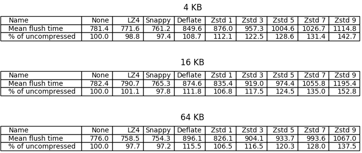
The first benchmark measures disk space taken by SSTables. Running a fresh ScyllaDB instance on 3 shards I inserted the data, flushed the memtables, and measured the size of the SSTable directory. Here are the results.
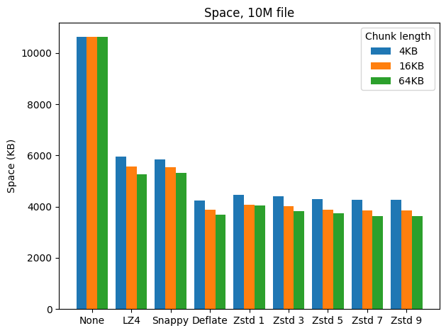
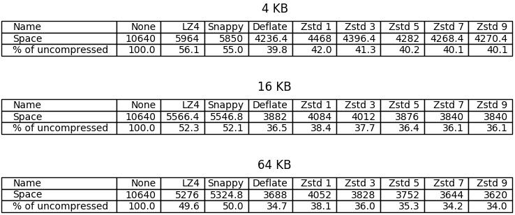
The best compression ratios were achieved with DEFLATE and higher levels of ZStandard. LZ4 and Snappy performed great too, halving the space taken by uncompressed tables when 64 KB chunk lengths were used. Unfortunately the differences between higher levels of ZStandard are pretty insignificant in this benchmark, which should not be surprising considering the small sizes of chunks used; it can be seen though that the differences grow together with chunk length.
Compression speed
The purpose of the next benchmark is to compare compression speed. I did the same thing as in the first benchmark, except now I measured the time it took to flush the memtables and repeated the operation ten times for each compression setting. On the error bar below, dots represent means and bars represent standard deviations.
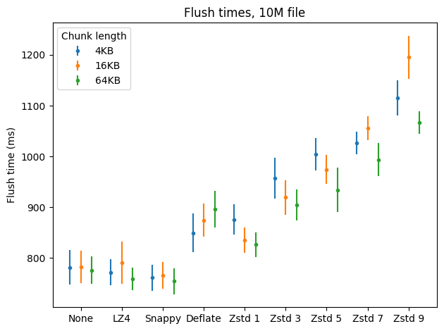
What I found most conspicuous was that flushing was sometimes faster when using LZ4 and Snappy compared to no compression. The first benchmark provides a possible explanation: in the uncompressed case we have to write twice the amount of data to disk than in the LZ4/Snappy case, and writing the additional data takes longer than compression (which happens in memory, before SSTables are written to disk), even with fast disks (my benchmarks were running on top of an M.2 SSD drive).
Another result that hit my eye was that in some cases compression happened to be significantly slower for 16KB chunks. I don’t have an explanation for this.
It looks like ZStandard on level 1 put up a good fight, being only less than 10 percentage points behind LZ4 in the 64KB case, followed by DEFLATE which performed slightly worse in general (the mean was better in the 4KB case, but there’s a big overlap when we consider standard deviations). Unfortunately ZStandard became significantly slower with higher levels.
Decompression speed
Let’s see how decompression affects the speed of reading from SSTables. I first inserted the data for each tested compression setting to a separate table, restarted ScyllaDB to clean the memtables, and performed a select * from each table, measuring the time; then repeated that last part nine times. Here are the results.
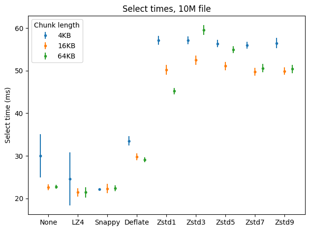
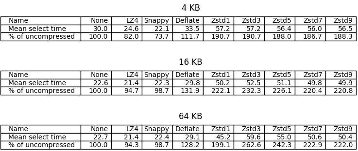
In this case ZStandard even on level 1 behaves (much) worse than DEFLATE, which in turn is pretty close to what LZ4 and Snappy offer. Again, as before, reading compressed files is faster with LZ4/Snappy than in the uncompressed case, possibly because the files are simply smaller.
Interestingly, using greater chunks makes reading faster for most of the tested algorithms.
Reactor stalls
The last benchmark measures the number and length of reactor stalls. Let me remind you that ScyllaDB runs on top of Seastar, a C++ framework for asynchronous programing. Applications based on Seastar have a sharded, “shared-nothing” architecture, where each thread of execution runs on a separate core which is exclusively used by this thread (if we take other processes in the system out of consideration). A Seastar programmer explicitly defines units of work to be performed on a core. The machinery which schedules units of work on a core in Seastar is called the reactor.
For one unit of work to start, the previous unit of work has to finish; there is no preemption happening as in classical threaded environment. It is the programmer’s job to keep units of work short — if they want to perform a long computation, then instead of doing it in a single shot, they should perform a part of it and schedule the rest for the future (in a programming construct called a “continuation”) so that other units have the chance to execute. When a unit of work computes for an undesirably long time, we call that situation a “reactor stall”.
When does a computation become “undesirably long”? That depends on the use case. Sometimes ScyllaDB is used as a data warehouse, where the number of concurrent requests to the database is low; in that case we can give ourselves a little leeway. Many times ScyllaDB is used as a real-time database serving millions of requests per second on a single machine, in which case we want to avoid reactor stalls like the plague.
The compression algorithms used in ScyllaDB weren’t implemented from scratch by ScyllaDB developers — there is little point in doing that. We are using the available fantastic open source implementations often coming from the authors of the algorithms themselves. A lot of work was put into these implementations to make sure they are correct and fast. However, using external libraries comes with a cost: we temporarily lose control over the reactor when we call a function from such a library. If the function is costly, this might introduce a reactor stall.
I measured the counts and lengths of reactor stalls that happen during SSTable flushes performed for the first two benchmarks. Any computation that took 1ms or more was considered a stall. Here are the results.
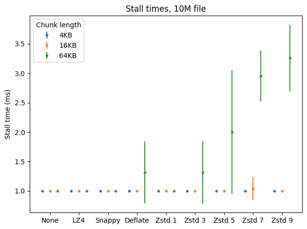
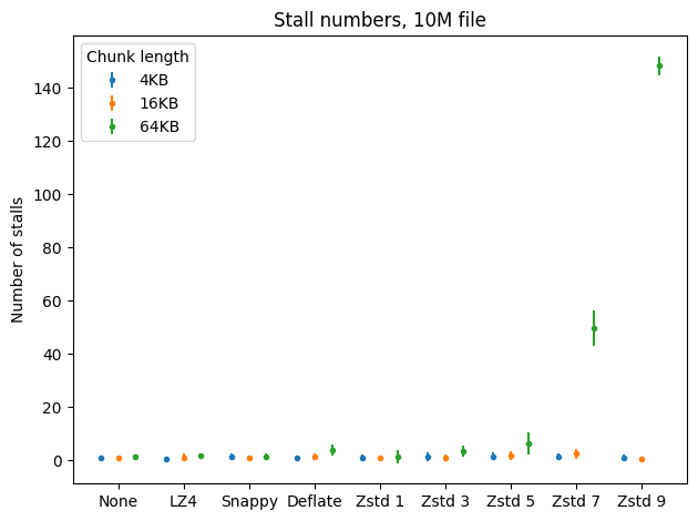
Fortunately reactor stalls aren’t a problem with the fast algorithms, including ZStandard on level 1. They sometimes appear when using DEFLATE and higher levels of ZStandard, but only with greater chunk lengths and still not too often. In general the results are pretty good.
Part 2 Conclusions
Use compression. Unless you are using a really (but REALLY) fast hard drive, using the default compression settings will be even faster than disabling compression, and the space savings are huge.
When running a data warehouse where data is mostly being read and only rarely updated, consider using DEFLATE. It provides very good compression ratios while maintaining high decompression speeds; compression can be slower, but that might be unimportant for your workload.
If your workload is write-heavy but you really care about saving disk space, consider using ZStandard on level 1. It provides a good middle-ground between LZ4/Snappy and DEFLATE in terms of compression ratios and keeps compression speeds close to LZ4 and Snappy. Be careful however: if you often want to read cold data (from the SSTables on disk, not currently stored in memory, so for example data that was inserted a long time ago), the slower decompression might become a problem.
Remember, the benchmarks above are artificial and every case requires dedicated tests to select the best possible option. For example, if you want to decrease your tables’ disk overhead even more, perhaps you should consider using even greater chunk lengths where higher levels of ZStandard can shine — but always run benchmarks first to see if that’s better for you.