Why Database Sizing is Hard

Adventures in building a performance model for a database
Sizing is something that seems deceptively simple: take the size of your dataset and the required throughput and divide by the capacity of a node. Easy, isn’t it?
If you’ve ever tried your hand at capacity planning, you know how hard it can be. Even making rough estimation can be quite challenging. Why is this so hard?
Let us detail the steps of estimating the size of a cluster:
- Make assumptions about usage patterns
- Estimate the required workload
- Decide on high level configuration of the database
- Feed the workload, configurations and usage patterns to a performance model of the database
- Profit!
This recipe, while easy to read, isn’t so simple to follow in practice. For example, when making decisions on database configuration, e.g. replication factor and consistency levels — your decisions are influenced by a preconceived notion of the answer. When cost becomes prohibitively expensive, suddenly those 5 replicas we wanted seem to be a bit of an overkill, don’t they? Thinking about sizing as a design process, we realize that it must be iterative, and support discovery and research of the requirements and usage. And like any design process, sizing is also limited in the time and resources we can devote to it — when optimal technical sizing is neither economically practical nor operationally desired. There is an inherent tradeoff between the simplicity and cost of the design process and accuracy; after all, a model sophisticated enough to predict database performance with high fidelity might be as costly as building the database itself, and require so many inputs as to be impractical to use!
How Many Romans?

When your boss asks why your sizing calculations were off…
The workload of a database is often described as the throughput of queries and the dataset size that it must support. This immediately raises some questions:
- Is this number the maximum throughput or an average? (Workloads often have periodical variation and peaks)
- Should we separate certain types of queries? (e.g. reads and writes)
- How do we estimate the number queries if we are not yet using this database? The size of the dataset?
- What is the hot dataset? Databases can store vastly more data than they can actively serve at any given point in time
- What about data models? We know from experience that data models have a large impact on the number of queries, performance and storage size
- What is the expected growth? You want to build a database that can scale with your workload
- What is the SLO of the queries? What latency targets are we designing for?
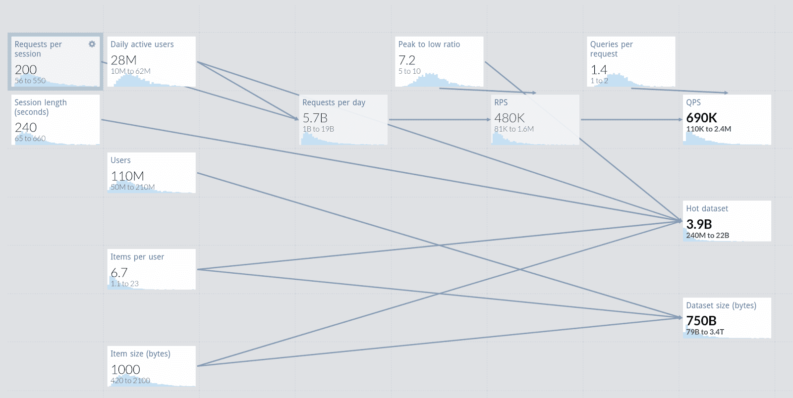
Some people are fortunate enough to have a working system, perhaps with a similar database, from which they can easily extract or extrapolate answers to some of these questions. But generally, we are forced to use guesstimation methods and back of the envelope calculations. This is not as bad as it sounds! For example, have a look at this model which uses the Monte-Carlo tool getguesstimate.
Workload estimation is interesting enough to merit a blog post of its own. But for the purposes of simple sizing, we are interested in the maximum values of throughput and dataset and will make a distinction between only two types of queries: reads and writes, for reasons that will be explained later. We can also assume that we control the data model to a high degree; as for any NoSQL database, our goal is to design such that we can handle all required data with a single query — we will need to make a decision if we want to optimize for reads or writes.
Usually, the basic steps would be:
- Estimate your peak dataset size and workload
- Sketch a preliminary data model, making high level decisions about optimization target
- Estimate the read/write ratio based on your data model
Building a database performance model

“All models are wrong, but some are useful” — attributed to George E. P. Box
(Image source: UPC)
To be useful, a Scylla performance model must balance between a few sometimes conflicting requirements: It must take ample performance and capacity safety margins, yet not present prohibitive cost, reliability vs performance, sustained and peak load. It must balance all of these yet still be simple enough to use even without a specific application in mind, while providing realistic results.
This is a challenging task indeed, but thankfully Scylla makes it easier as it scales pretty linearly with the addition of cores and nodes. All we need to do is predict how many operations a CPU core can handle…
Queries vs operations
The workload is specified in terms of queries, usually CQL. CQL queries can be quite complex and generate a varying number of “primitive operations” whose performance is relatively predictable. Take for example the following CQL queries:
SELECT * FROM user_stats WHERE id=UUIDSELECT * FROM user_stats WHERE username=USERNAMESELECT * FROM user_stats WHERE city=”New York” ALLOW FILTERING
Query #1 will locate records using a primary key and thus be immediately executed on the correct partition — it might still break down to several operations as, depending on the consistency level, several replicas will be queried (more on that later).
Query #2, despite looking quite similar, happens to lookup records based on a secondary index, breaking down to two subqueries: one to the global secondary index to find the primary key and another one to retrieve the row from the partition. Plus again, depending on the consistency level, this might generate several operations.
Query #3 is even more extreme, as it scans across partitions; its performance will be bad and unpredictable.
Another example is UPDATE queries:
UPDATE user_stats SET username=USERNAME, rank=231, score=3432 WHERE ID=UUIDUPDATE user_stats SET username=USERNAME, rand=231, score=3432 WHERE ID=UUID IF EXISTS
Query #1 may intuitively appear to break down to 2 operations — read and write — but in CQL UPDATE queries are UPSERT queries and only 1 write operation will be generated.
Query #2 however, despite looking similar, will not only require read-before-write on all replicas but also Lightweight Transactions (LWTs) which requires expensive orchestration.
Similarly, the amount of disk operations generated by a query can vary significantly. Scylla uses Log Structured Merge tree (LSM) structures in a Sorted Strings Table (SSTable) storage format. Scylla never modifies SSTable files on disk; they are immutable. Writes are persisted to an append-only commit log for recovery and are written to a memory buffer (memtable). When the memtable becomes too large, it gets written to a new SSTable file on disk and flushed from memory. This makes the write path extremely efficient, but introduces a problem with reads: Scylla must search multiple SSTables for a value.
To prevent this read amplification from going out of control Scylla periodically compacts multiple SSTables into a smaller number of files, keeping only the most current data. This reduces the amount of read operations required to complete a query. (Read more about Scylla’s compaction operations and various compaction strategies in our documentation here.)
What this means is that attributing disk operations to a single query is practically impossible. The exact number of disk operations depends on the number of SSTables, their arrangement, the compaction strategy etc. Fortunately, Scylla is designed to squeeze the maximum out of your storage, so as long as the disks are fast enough and are not the bottleneck, we can ignore this dimension. This is why we recommend fast NVMe local disks.
While this example focuses on CQL, the problem of predicting query cost is not unique. In fact, the richer and powerful the query language the harder it is to predict its performance. SQL performance for example, because of it’s tremendous power, can be very unpredictable. Sophisticated query optimizers are therefore an essential part of RDBMS and do improve performance, at the cost of making performance even harder to predict. This is another tradeoff where NoSQL takes a very different route: preferring predictable performance and scalability over rich query languages.
The Consistency Conundrum
Scylla, being a distributed and highly available database, needs to reliably replicate data to several nodes. The number of replicas is configurable per keyspace and known as Replication Factor. From the point of view of the client, this can happen synchronously or asynchronously, depending on the Consistency Level of the write. For example, when writing with consistency level ONE, data will be eventually written to all replicas, but the client will only wait for one replica to acknowledge the write. Even if some of the nodes are temporarily unavailable, Scylla will cache writes and replicate later when these nodes are available (this is known as Hinted Handoff). In practice we can assume that every write query will generate at least one write operation on every replica.
For reads however, the situation is somewhat different. A query with consistency level ALL must read from all replicas, thus generating as many read operations as your cluster’s Replication Factor, but a query with consistency level ONE will only read from a single node allowing for cheaper and faster reads. This allows users to squeeze more read throughput out of their cluster at the expense of consistency, because that one node may not yet have gotten the latest update when it is read.
Finally, there is LWT to consider. As mentioned before, LWT required orchestration throughout all replicas utilizing the Paxos algorithm. Not only does LWT force each replica to read then write the value, it also needs to maintain the state of the transaction until the Paxos round is complete. Because of the different way LWT behaves we treat it as a separated performance model for the throughput each core can support.
All operations are equal, but some are more equal than others
Now that we have broken down CQL queries to primitive operations, we can ask how much time (and resources) each operation takes? What is the capacity a CPU core can support? Again, the answer is somewhat complicated. As an example, let’s consider a simple read and follow the execution steps within a node:
- Lookup the value in the memory table. If not found…
- Lookup the value in the cache. If not found…
- Lookup the value in SSTables, level by level and merge the values
- Respond to the coordinator
Clearly, reads will complete much faster if they are in the RAM-based memtable or row-level cache; nothing surprising about that. Additionally steps #3 and #4 can incur higher cost depending on the size of the data being read from disk, processed and transferred over the network. If we need to read 10MB of data, this may take considerable time. This can happen either because the values stored in individual cells are large or because a range scan returns many results. However, in the case of large values, Scylla cannot chunk them into smaller pieces and must load the entire cell to memory.
In general, it is advisable to model your data such that partitions, rows and cells do not grow too large to ensure low variance of performance, but in reality there will always be some variance. Read this article about how you can locate and troubleshoot large rows and cells in Scylla.
This variance is especially problematic when it comes to partition access patterns. The strategy many databases use to scale and spread data across nodes is to chunk data into partitions which are independent of each other. But being independent also means partitions may experience uneven load, leading to what is known as the “hot partition” problem – where a single partition hits node capacity limits despite the rest of the cluster having ample resources. The occurrence of this problem highly depends on the data model, the distribution of partition keys in the dataset and the distribution of keys in the workload. As predicting hot partitions generally requires analyzing the entire dataset and workload and therefore impractical at the design phase, we can supply certain well known distributions as input to our model, or make some assumptions about the relative heat of partitions. We also provide the nodetool toppartitions command to help you locate the hot partitions in your Scylla database.
Materialized views, Secondary indexes and other magical beasts
Like many other databases, Scylla features automatic secondary indexes and materialized views as well as Change Data Capture (CDC). These are essentially secondary tables which are maintained by the database itself, and allow writing data in multiple forms using only one write operation. Under the hood, Scylla derives new values to be written according to the schema provided by the user and writes these new values to a different table. The main differences between Scylla and RDBMS in that regard is that the derived data is written asynchronously and across the network as indexes and materialized views are not limited to a single partition. This is another source of write amplification we should consider, but thankfully in Scylla it is rather predictable and similar in performance to user generated operations. For every item written, one write will be triggered for CDC and each materialized view or secondary index derived from the written cells. In some cases, materialized views and CDC might require an additional read, this can happen for example if the CDC “preimage” or “postimage” features are enabled. Also, remember that a single CQL query can trigger multiple write operations.
CDC, secondary indexes and materialized views are implemented as regular tables managed by Scylla itself, but that also means they consume a comparable amount of disk space to user tables, which we must account for in our capacity plan.
Peaks and the art of database maintenance
All databases have various maintenance operations they must perform. RDBMS need to cleanup redo logs (e.g. the notorious PostgreSQL VACUUM), dump a snapshot to disk (looking at your Redis), or perform memory garbage collection (Cassandra, Elastic, HBase). Databases which use LSM storage (such as Cassandra, HBase and Scylla) also need to periodically compact SSTables and flush memtables into new SSTables. You can get top performance for a short time as Scylla is intelligent enough to postpone maintenance operations such as compaction and repair to a later, less overloaded time; But eventually you will have to spare resources for these maintenance operations to be done. This is very useful for most systems as load is rarely uniform across the day, but our plan should allow for enough capacity for sustained long lasting operation of the database.
Additionally, planning based on throughput alone is insufficient. To some extent, you can overload the database to achieve higher throughput at the cost of higher latency.
Benchmarks are often misleading in that sense, usually too short to reach meaningful sustained operation. Latency/throughput tradeoff is usually easier to measure and can be observed even in short benchmarks.
Another important yet often overlooked matter is degraded operation. Being a natively redundant and highly available database Scylla is designed to smoothly handle node failures (according to consistency constraints set by the user). But while failures are semantically coherent this does not mean they are dynamically transparent — a significant loss of capacity will affect the performance of the cluster, as well as the restoration or replacement of the failed node. These too need to be accounted for when sizing the cluster.
The Commando and the Legion
As Scylla capacity can be increased both by adding nodes or by choosing larger nodes, an interesting question arises: which scaling strategy should be chosen? On the one hand, larger nodes are more efficient as we can allocate CPU cores to deal with network and other OS level tasks independently from the cores serving Scylla, as well as reduce the relative overhead of node coordination. On the other hand the more nodes you have, the less fractional capacity you lose when one fails — although the probability of losing a node is somewhat higher.
For very large workloads, this question is moot as large nodes are simply not enough. But for many smaller workloads, owing to the extreme performance of Scylla, 3 medium-large nodes can be quite enough. This decision is contextual for your workload, but for reliable degraded operation it is recommended to run at least 6-9 nodes (assuming replication factor 3).
Conclusion
Capacity planning and sizing your cluster can be quite complex and challenging. We’ve talked about how you should take into account your safety margins, maintenance operations and usage patterns. It is important to remember that any guesstimation is only an initial estimate to iterate on. Once you get into production and have real numbers, let that guide your capacity planning. Your Mileage Will Vary.
If you’ve enjoyed reading this article, you may also appreciate this blog from my colleague Eyal Gutkind on Sizing Up Your Scylla Cluster.
As always, we are happy to receive community feedback, either contact us directly, or raise your issues in our community Slack channel.