Migrating from Postgres to ScyllaDB, with 349X Faster Query Processing
How Coralogix cut processing times from 30 seconds to 86 milliseconds with a PostgreSQL to ScyllaDB migration
Speed matters for Coralogix, an observability platform that dev teams trust to spot incidents before they escalate into problems. Coralogix uses a real-time streaming analytics pipeline, providing monitoring, visualization, and alerting capabilities without requiring indexing.
One of Coralogix’s key differentiators is a distributed query engine for fast queries on mapped data from a customer’s archives in remote storage. That engine queries semi-structured data stored in object storage (e.g., GCS, S3) using a specialized Parquet format. It was originally designed as a stateless query engine on top of the underlying object storage, but reading Parquet metadata during query execution introduced an unacceptable latency hit. To overcome this, they developed a metadata store (simply called “metastore”) to enable faster retrieval and processing of the Parquet metadata needed to execute large queries.
The original metastore implementation, built on top of PostgreSQL, wasn’t fast enough for their needs. So, the team tried a new implementation – this time, with ScyllaDB instead of PostgreSQL. Spoiler: It worked. They achieved impressive performance gains – cutting query processing time from 30 seconds to 86 milliseconds. And their engineers Dan Harris (Principal Software Engineer) and Sebastian Vercruysse (Senior Software Engineer) took the stage at ScyllaDB Summit to explain how they did it. This article is based on their presentation.
Join us at ScyllaDB Summit 24 to hear more firsthand accounts of how teams are tackling their toughest database challenges. Disney, Discord, Expedia, Supercell, Paramount, and more are all on the agenda.
Metastore Motivation and Requirements
Before getting into the metastore implementation details, let’s take a step back and look at the rationale for building a metastore in the first place.
“We initially designed this platform as a stateless query engine on top of the underlying object storage – but we quickly realized that the cost of reading Parquet metadata during query execution is a large percentage of the query time,” explained Dan Harris. They realized that they could speed this up by placing it in a fast storage system that they could query quickly (instead of reading and processing the Parquet metadata directly from the underlying object storage).
They envisioned a solution that would:
- Store the Parquet metadata in a decomposed format for high scalability and throughput
- Use bloom filters to efficiently identify files to scan for each query
- Use transactional commit logs to transactionally add, update, and replace existing data in the underlying object storage
Key requirements included low latency, scalability in terms of both read/write capacity, and scalability of the underlying storage. And to understand the extreme scalability required, consider this: a single customer generates 2,000 Parquet files per hour (50,000 per day), totaling 15 TB per day, resulting in 20 GB in Parquet metadata alone for a single day.
The Initial PostgreSQL Implementation
“We started the initial implementation on Postgres, understanding at the time that a non-distributed engine wouldn’t be sufficient for the long run,” Dan acknowledged. That original implementation stored key information such as “blocks,” representing one row group and one Parquet file. This includes metadata like the file’s URL, row group index, and minimal details about the file. For example:
Block url:
s3://cgx-production-c4c-archive-data/cx/parquet/v1/team_id=555585/…
…dt=2022-12-02/hr=10/0246f9e9-f0da-4723-9b64-a12346095d25.parquet
Row group: 0, 1, 2 …
Min timestamp
Max timestamp
Number of rows
Total size
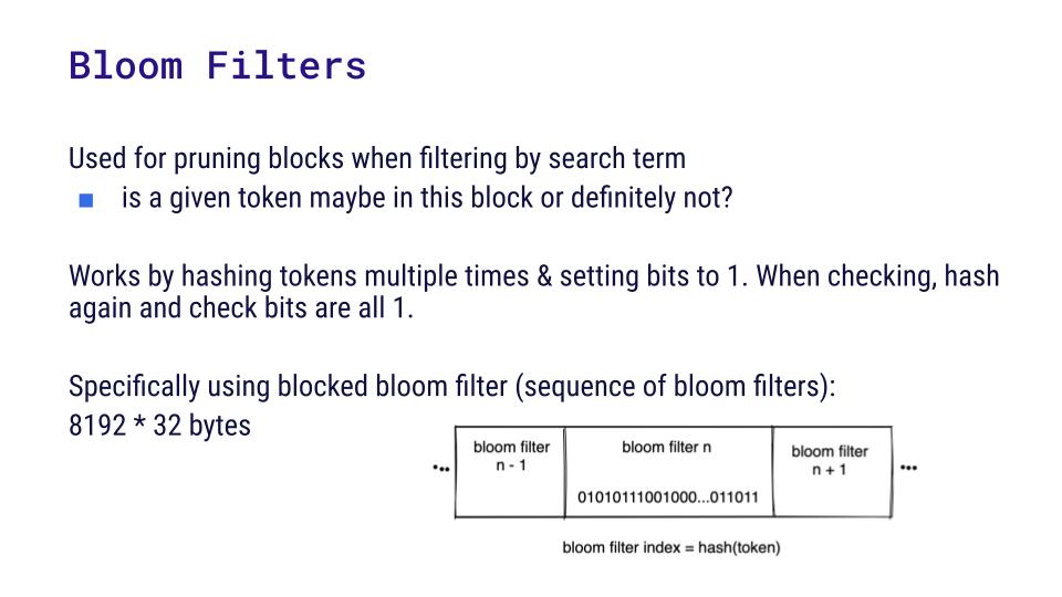
…To optimize reading, they used bloom filters for efficient data pruning. Dan detailed, “Eventually, we want to support something like full-text search. Basically, when we’re ingesting these files into our system, we can build a bloom filter for all the distinct tokens that we find in the file. Then, based off a particular query, we can use those bloom filters to prune the data that we need to scan.” They stored bloom filters in a block-split setup, breaking them into 32-byte blocks for efficient retrieval. They’re stored independently so the system doesn’t have to read the entire bloom filter at query time.
Additionally, they stored column metadata for each Parquet file. For example:
Block URL
Row Group
Column Name
Column metadata (blob)
Dan explained: “The files that we’re writing are quite wide, sometimes as many as 20,000 columns. So, by reading only the metadata that we need, we can really reduce the amount of IO required on any given query.”
ScyllaDB Implementation
Next, let’s look at the ScyllaDB implementation as outlined by Dan’s teammate, Sebastian Vercruysse.
Blocks Data Modeling
The block modeling had to be revisited for the new implementation. Here’s an example of a block URL:
s3://cgx-production-c4c-archive-data/cx/parquet/v1/team_id=555585/…
…dt=2022-12-02/hr=10/0246f9e9-f0da-4723-9b64-a12346095d25.parquet
The bold part is the customer’s top-level bucket; inside the bucket, items are partitioned by hour. In this case, what should be used as the primary key?
- (Table url)? But some customers have many more Parquet files than other customers, and they wanted to keep things balanced
- ((Block url, row group))? This uniquely identifies a given block, but it would be difficult to list all the blocks for a given day because the timestamp is not in the key
- ((Table url, hour))? That works because if you have 24 hours to query, you can query quite easily
- ((Table url, hour), block url, row group)? That’s what they selected. By adding the block url and row group as clustering keys, they can easily retrieve a specific block within an hour, which also simplifies the process of updating or deleting blocks and row groups.
Bloom Filter Chunking and Data Modeling
The next challenge: how to verify that certain bits are set, given that ScyllaDB doesn’t offer out-of-the-box functions for that. The team decided to read bloom filters and process them in the application. However, remember that they are dealing with up to 50,000 blocks per day per customer, each block containing 262 KB for the bloom filter part. That’s a total of 12 GB – too much to pull back into the application for one query. But they didn’t need to read the whole bloom filter each time; they needed only parts of it, depending on the tokens involved during query execution. So, they ended up chunking and splitting bloom filters into rows, which reduced the data read to a manageable 1.6 megabytes.
For data modeling, one option was to use ((block_url, row_group), chunk index) as the primary key. That would generate 8192 chunks of 32 bytes per bloom filter, resulting in an even distribution with about 262 KB per partition. With every bloom filter in the same partition, it would be easy to insert and delete data with a single batch query. But there’s a catch that impacts read efficiency: you would need to know the ID of the block before you could read the bloom filter. Additionally, the approach would involve accessing a substantial number of partitions; 50K blocks means 50K partitions. And as Sebastian noted, “Even with something as fast as ScyllaDB, it’s still hard to achieve sub-second processing for 50K partitions.”
Another option (the one they ultimately decided on): ((table url, hour, chunk index), block url, row group). Note that this is the same partition key as the Blocks one, with an added index to the partition key that represents the nth token required by the query engine. With this approach, scanning 5 tokens spanning a 24 hour window results in 120 partitions – an impressive improvement compared to the previous data modeling option.
Furthermore, this approach no longer requires the block ID before reading the bloom filter – allowing for faster reads. Of course, there are always trade-offs. Here, due to the blocked bloom filter approach, they have to split a single bloom filter into 8192 unique partitions. This ends up impacting the ingestion speed compared to the previous partitioning approach that allowed ingesting all bloom filter chunks at once. However, the ability to quickly read a given block within an hour is more important to them than fast writes – so they decided that this tradeoff was worth it.
Data Modeling Woes
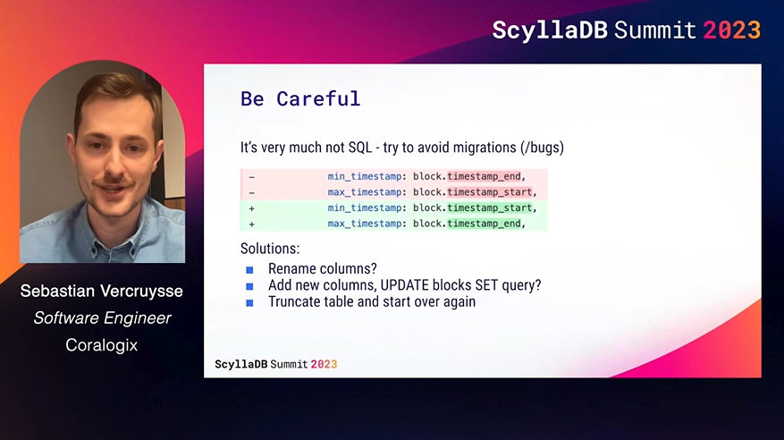
Not surprisingly, moving from SQL to NoSQL involved a fair amount of data modeling rework, including some trial and error. For example, Sebastian shared, “One day, I figured out that we had messed up min and max timestamps – and I wondered how I was going to fix it. I thought maybe I could rename the columns and then somehow make it work again. But, here you cannot rename a column if it’s part of a clustering key. I thought I could perhaps add new columns and run an UPDATE query to update all rows. Unfortunately, this doesn’t work in NoSQL either.”
Ultimately, they decided to truncate the table and start over again vs writing migration code. Their best advice on this front is to get it right the first time. 🙂
Performance Gains
Despite the data modeling work required, the migration paid off nicely. For the metastore block listing:
- Each node currently handles 4-5 TB.
- They’re currently processing around 10K writes per second with P99 latency consistently below one millisecond.
- The block listing results in about 2000 parquet files in an hour; with their bloom filters, they’re processed in less than 20 milliseconds.
- For 50K files, it’s less than 500 milliseconds.
They also do checking of bits. But, for 50K Parquet files, 500 milliseconds is fine for their needs.
In the column metadata processing, the P50 is quite good, but there’s a high tail latency. Sebastian explained: “The problem is that if we have 50K Parquet files, our executors are fetching all of these in parallel. That means we have a lot of concurrent queries and we’re not using the best disks. We assume that’s at the root of the problem.”
ScyllaDB Setup
Notably, Coralogix moved from first discovering ScyllaDB to getting into production with terabytes of data in just 2 months (and this was a SQL to NoSQL migration requiring data modeling work, not a much simpler Cassandra or DynamoDB migration).
The implementation was written in Rust on top of the ScyllaDB Rust driver, and they found ScyllaDB Operator for Kubernetes, ScyllaDB Monitoring, and ScyllaDB Manager all rather helpful for the speedy transition. Since offering their own customers a low-cost observability alternative is important to Coralogix, the Coralogix team was pleased by the favorable price-performance of their ScyllaDB infrastructure: a 3-node cluster with:
- 8 vCPU
- 32 GiB memory
- ARM/Graviton
- EBS volumes (gp3) with 500 MBps bandwidth and 12k IOPS
Using ARM reduces costs, and the decision to use EBS (gp3) volumes ultimately came down to availability, flexibility, and price-performance. They admitted, “This is a controversial decision – but we’re trying to make it work and we’ll see how long we can manage.”
Lessons Learned
Their key lessons learned here…
Keep an eye on partition sizes: The biggest difference in working with ScyllaDB vs working with Postgres is that you have to think rather carefully about your partitioning and partition sizes. Effective partitioning and clustering key selection makes a huge difference for performance.
Think about read/write patterns: You also have to think carefully about read/write patterns. Is your workload read-heavy? Does it involve a good mix of reads and writes? Or, is predominantly write-heavy? Coralogix’s workloads are quite write-heavy because they’re constantly ingesting data, but they need to prioritize reads because read latency is most critical to their business.
Avoid EBS: The team admits they were warned not to use EBS: “We didn’t listen, but we probably should have. If you’re considering using ScyllaDB, it would probably be a good idea to look at instances that have local SSDs instead of trying to use EBS volumes.”
Future Plans: WebAssembly UDFs with Rust
In the future, they want to find the middle ground between writing large enough chunks and reading unnecessary data. They’re splitting the chunks into ~8,000 rows and believe they can split them further into 1,000 rows, which could speed up their inserts.
Their ultimate goal is to offload even more work to ScyllaDB by taking advantage of User Defined Functions (UDFs) with WebAssembly. With their existing Rust code, integrating UDFs would eliminate the need to send data back to the application, providing flexibility for chunking adjustments and potential enhancements.
Sebastian shares, “We already have everything written in Rust. It would be really nice if we can start using the UDFs so we don’t have to send anything back to the application. That gives us a bit more leeway to play with the chunking.”
Watch the Complete Tech Talk
You can watch the complete tech talk and skim through the deck in our tech talk library.